Point Cloud Representations and Voxelization: First Principles
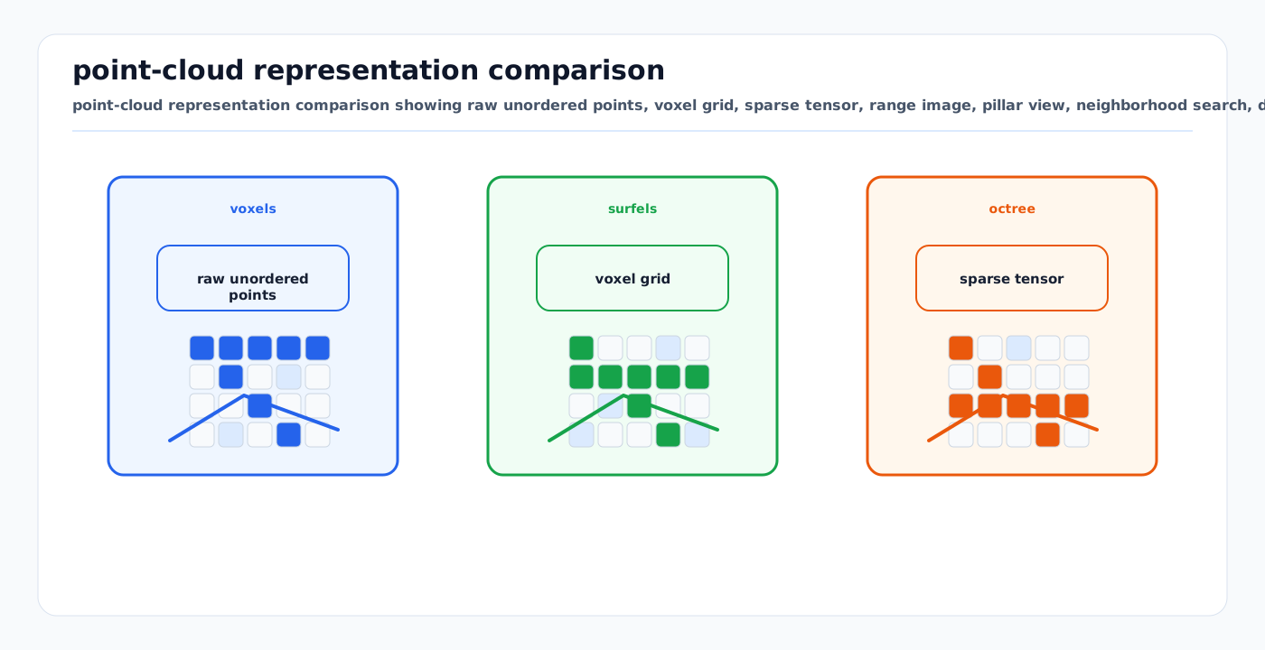
Visual: point-cloud representation comparison showing raw unordered points, voxel grid, sparse tensor, range image, pillar view, neighborhood search, devoxelization, and aggregated-map suitability.
A LiDAR point cloud is a finite, unordered set of 3D measurements with no canonical spatial structure. Every downstream architecture — sparse CNN, point-based network, range-image model, or hybrid — depends critically on how raw returns are organized before features are extracted. Representation choice determines memory cost, geometric fidelity, sensor compatibility, and whether the resulting data structure is valid for aggregated multi-scan maps or only for ego-centric single sweeps.
Related Docs
- Point Cloud Segmentation Losses and Metrics: First Principles
- LiDAR Working Principles and Noise Models
- Point Cloud Registration: ICP, NDT, GICP
- Correspondence Search and Data Structures
- Sparse Attention for 3D Perception
Why It Matters
| Choice | Effect | Risk if wrong |
|---|---|---|
| Raw points vs. voxels | Exact geometry vs. discretized grid. | Voxels alias thin structures; points are slow on large maps. |
| Cartesian vs. cylindrical partition | Uniform cell size vs. sensor-density-matched cell size. | Cartesian wastes 99%+ memory on distant empty space; cylindrical breaks for aggregated maps. |
| Range image vs. 3D representation | 2D CNN efficiency vs. full 3D structure. | Range image is undefined for multi-scan maps; 3D required for accumulated point sets. |
| Pillar encoding | Fast 2D CNN path; height compressed. | Vertical structure (overpass, stacked cargo, jetway) is lost; unsuitable for full 3D semantic labeling. |
| Voxel size | Resolution ↔ memory ↔ speed balance. | Too coarse: thin objects (bollards, signage poles) disappear into background voxels. |
| Devoxelization strategy | How voxel-space features return to per-point predictions. | Nearest-voxel lookup preserves quantization error; trilinear interpolation recovers sub-voxel resolution. |
Raw Point Sets
Nature of the Data
A LiDAR sweep is a finite unordered set S = {p1, p2, ..., pN} where each point pi is a vector in R^D. The physical firing order (return index, beam sequence) carries no semantic meaning; the set is permutation-invariant by construction. This is the foundational representational challenge: most deep learning operators assume structured grids or sequences with a canonical ordering.
Per-point feature channels (D dimensions) typically include:
(x, y, z)              -- Cartesian coordinates, always present (3 dims)
intensity/reflectance  -- LiDAR return amplitude; material discriminator (1 dim)
normal vector (nx,ny,nz) -- estimated surface normal; planarity reasoning (3 dims)
timestamp / ring-id    -- firing time or laser beam index; motion de-skewing (1-2 dims)
RGB                    -- camera-fused color; optional (3 dims)
PointNet: Canonical Raw-Point Operator
PointNet (Qi et al., CVPR 2017) resolved permutation invariance with a theoretically grounded approximation theorem: any continuous set function f: 2^R^N -> R can be arbitrarily approximated by:
f({x1,...,xN}) ≈ gamma( g( h(x1), h(x2), ..., h(xN) ) )where h is a shared MLP applied independently to each point, g is a symmetric aggregation function (max-pooling), and gamma is another MLP applied to the aggregated global descriptor.
Why max-pooling beats average-pooling: The global descriptor is determined by a small subset of "critical points" — those achieving the maximum in each feature dimension. This yields robustness to missing data and outliers (Theorem 2, PointNet paper). Average-pooling dilutes geometric signal.
Feature alignment (T-nets): Mini-networks predict 3x3 and 64x64 transformation matrices applied to input coordinates and mid-layer features. An orthogonality regularizer stabilizes feature-space alignment:
L_reg = || I - A * A^T ||_F^2Segmentation head: Per-point features from early layers are concatenated with the global max-pooled descriptor, then decoded per-point to class logits.
Limitations: PointNet's symmetric pooling collapses local neighborhood structure. PointNet++ addresses this with hierarchical set abstraction and ball-query grouping. KPConv and PointTransformer extend further with learned or attention-based local operators.
Architecture family: PointNet → KPConv → RandLA-Net → PointTransformerV3 all operate on raw point sets without discretization. RandLA-Net achieves 1M-point processing via random downsampling combined with attentive aggregation.
Voxel Grids
Dense Voxel Grids and the Cubic-Memory Problem
A dense voxel grid partitions a 3D bounding volume into a regular W x H x D array of cubic cells. Memory scales as O(W * H * D).
Example: 10 cm resolution, 100 m x 100 m x 5 m volume
W = 1000, H = 1000, D = 50
Total cells = 50,000,000
LiDAR occupancy rate: 0.1-1%
Empty cells: 99%+
Storing the full grid wastes nearly all memory on unoccupied space.
Sparse Voxels: Only Occupied Cells
Key insight: allocate memory and compute only for non-empty voxels. The sparse representation stores a list of (coordinates, features) pairs rather than a dense tensor.
Data structure — hash table / coordinate map (MinkowskiEngine):
Coordinates (x_int, y_int, z_int, batch_id) are hashed (e.g., FNV64-1A)
Hash map: occupied voxel key -> feature vector index
Kernel map: precomputes input-output voxel neighbor relations per convolution
Generalized sparse convolution (Choy et al., MinkowskiEngine):
x_u_out = sum_{i in kernel_offsets} W_i * x_{u+i}_in
                                     (only where u+i is in C_in)
Arbitrary input/output coordinate sets C_in, C_out are supported, encompassing transposed (expanding) and contracting (downsampling) convolutions.
Submanifold Sparse Convolution
Submanifold constraint: C_out = C_in. Output occupancy pattern exactly matches input — no new voxels are activated by a convolution pass. This prevents the "dilation problem" where repeated sparse convolutions fill in empty space.
Implementation: When C_out = C_in, the kernel map is built by querying each input coordinate's neighborhood in the hash table, recording only hits already present in C_in. The number of active voxels stays constant across all submanifold layers. This is the default operation in MinkowskiNet and spconv (used by VoxelNet, CenterPoint, SPVCNN).
Coordinate Systems for Voxelization
| Partition | Coordinate axes | Cell shape | LiDAR density match |
|---|---|---|---|
| Cartesian | (x, y, z) uniform | Cube | Poor — cells far from sensor are mostly empty |
| Cylindrical | (rho, theta, z) radius, azimuth, height | Wedge-shaped frustum | Good — cell volume grows with r, compensating for LiDAR 1/r^2 density fall-off |
| Spherical/polar | (r, phi, theta) | Solid angle section | Matches single-scan geometry exactly; pathological for multi-scan maps |
Cylinder3D / CA3D (Zhu et al., CVPR 2021) converts Cartesian (x,y,z) to cylindrical (rho, theta, z) then partitions uniformly in cylindrical space. Voxels near the sensor are small (high resolution where density is high); voxels far away are large (appropriately sized for sparse regions). Empirical result on SemanticKITTI:
Cylindrical partition: 89% non-empty cell occupancy
Cartesian partition:   61% non-empty cell occupancy
~6x improvement in occupancy balance at distant regions
Why cylindrical breaks for aggregated maps: Cylindrical coordinates are centered on a single sensor origin. An accumulated multi-scan map has no single origin. A cylinder partition referenced to one pose is misaligned for all other sensor positions in the map.
Why spherical/polar breaks for aggregated maps: Spherical projection assigns each measurement a unique (r, phi, theta) relative to the sensor. In a world-frame map with returns from thousands of poses, the azimuth/elevation reference frame is undefined — the projection produces conflicting or overlapping cells.
Pillars and Bird's-Eye-View
Lang et al. (CVPR 2019) proposed collapsing the z (height) dimension entirely, creating vertical columns (pillars) in the (x, y) plane.
Mechanics:
1. Divide x-y plane into W x H grid (e.g., 0.16 m resolution).
   Each cell is a pillar — an infinite-height column.

2. Collect all points falling in each pillar (max P points;
   empty pillars zero-padded; excess points randomly sampled).

3. Augment each point with offsets from pillar centroid (dx, dy, dz)
   and pillar center (xc, yc) -> 9 features total.

4. Shared PointNet MLP per-point within each pillar, then max-pooling
   -> single C-dim feature vector per pillar.

5. Scatter pillar features back to (x, y) grid -> dense pseudo-image
   of shape C x H x W.

6. Standard 2D CNN backbone + SSD-style detection head on pseudo-image.
BEV pseudo-image: The pillar encoding produces a bird's-eye-view feature map processed by highly optimized 2D convolution kernels, avoiding 3D sparse convolution overhead entirely.
Trade-off: All vertical structure is compressed into a single feature vector. Height-separated objects (overpass vs. road, stacked pallets, jetway connections vs. ground) may be confused. Pillar resolution is the key hyperparameter: Waymo typically uses 0.1 m; nuScenes 0.075 m.
Why pillars suit safety-path detectors: PointPillars achieves ~6.84 ms INT8 on NVIDIA Orin for the safety-path LiDAR detection pass — within the ~100 ms autonomy compute budget. Not suitable for full 3D semantic segmentation of complex airside geometry.
Range Images
Spherical Projection
A spinning LiDAR fires H laser beams at fixed elevation angles while rotating W azimuth steps per revolution. Each measurement (r, phi, theta) maps to a pixel in an H x W range image:
u = floor( (theta - theta_min) / (theta_max - theta_min) * W )   (azimuth column)
v = floor( (phi   - phi_min)   / (phi_max   - phi_min)   * H )   (elevation row)
pixel value: range r = sqrt(x^2 + y^2 + z^2)
Additional channels per pixel: intensity, derived (x,y,z), surface normal. The result is a structured 2D array amenable to standard 2D CNNs (ResNet, U-Net, DarkNet).
RangeNet++ (Milioto et al., IROS 2019): applies DarkNet53 backbone on the range image; uses a KNN post-processing step to propagate range-image labels back to 3D points, partially correcting discretization artifacts.
SalsaNext: U-Net-style encoder-decoder with dilated convolutions and uncertainty-aware heads; 7x fewer parameters than RangeNet++ with improved mIoU. Range image provides 2D grid structure; speed benefit is the primary advantage over 3D representations.
Limitations
Single-origin assumption: Each range image encodes data from one sensor position. The column index u corresponds to one full rotation. Multi-scan accumulated maps have no single azimuth/elevation reference frame — range image projection is undefined or produces overlapping/conflicting pixels.
Many-to-one collisions: Multiple 3D points can project to the same pixel (farther point occluded by closer one). KNN post-processing partially reassigns labels to occluded points, but the representation itself loses them.
Discretization (quantization) error: Angular resolution is fixed by beam count H. For 64 beams: ~0.4 degree elevation resolution. Points close together in 3D but slightly different in angle map to different rows; points far apart but at the same angle collide to the same row.
Sensor-specific grid: Range image dimensions are tied to a specific LiDAR model (Velodyne HDL-64E, Ouster OS2-128, etc.); changing sensor requires full retraining or remapping.
Octrees
Adaptive Hierarchical Subdivision
An octree recursively subdivides 3D space into 8 octants until each occupied leaf cell contains at most a threshold number of points or maximum depth is reached. Empty octants are pruned entirely. Memory is O(N_surface) in the number of occupied surface points, not O(resolution^3).
O-CNN (Wang et al., SIGGRAPH 2017) restricts CNN computation to octree nodes occupied by the 3D surface: "memory and computational costs grow quadratically as octree depth increases" — contrast with cubic growth for dense voxel grids.
OctFormer (Wang et al., ACM ToG 2023) extends the octree approach to transformers. Points are assigned to octree leaf nodes, then sorted by shuffled octree keys to partition points into local attention windows with a fixed number of points per window (not fixed spatial size). This guarantees consistent GPU utilization regardless of local density variation. Dilated octree attention expands the receptive field further.
OctFormer benchmark results (Wang et al. 2023):
- 17x faster than non-octree transformers at >200k points
- +7.3 mIoU over sparse-voxel CNNs on ScanNet200
Adaptive resolution advantage: Octrees allocate resolution where points are dense (near surfaces, near sensor) and coarsen where space is empty. This aligns with the multi-scale structure of real environments and the non-uniform density of LiDAR returns.
Superpoints and Superpoint Graphs
Geometric Over-Segmentation
Rather than operating on individual points (millions) or uniform voxels, superpoint methods partition the cloud into geometrically homogeneous regions called superpoints — analogous to superpixels in 2D segmentation.
SPG (Landrieu & Simonovsky, CVPR 2018) partitions via global energy minimization using the ℓ₀-cut pursuit algorithm solving a Potts model:
E = sum_i || f_i - s_i ||^2  +  lambda * |{ edges (i,j) : s_i != s_j }|

f_i  = per-point geometric features (linearity, planarity, scattering, verticality)
s_i  = superpoint assignment
lambda = regularization weight controlling partition coarseness
No pre-specification of the number of superpoints is required.
Superpoint shape features from PCA of constituent points:
lambda_1 >= lambda_2 >= lambda_3  (sorted eigenvalues of local covariance)

linearity  = (lambda_1 - lambda_2) / lambda_1
planarity  = (lambda_2 - lambda_3) / lambda_1
scattering = lambda_3 / lambda_1
Plus verticality and elevation.
Superpoint graph construction: Two superpoints are adjacent if their constituent points share a Voronoi edge. Edge attributes (13-dimensional) encode spatial offsets, standard deviations, centroid distances, and shape ratios between adjacent superpoints.
Classification pipeline (SPG):
1. Each superpoint -> PointNet embedding (128-point sample, rescaled to unit sphere)
2. GRU-based graph convolution over superpoint graph
   (T=10 iterations, Edge-Conditioned Convolutions with MLP-regressed weight vectors)
3. Concatenate hidden states -> linear classification head
SPT (Robert et al., ICCV 2023) modernizes SPG with a hierarchical partition P0 -> P1 -> P2 and a sparse self-attention transformer over superpoints. Key statistics:
SPT parameters:    212k   (vs. 41.6M for PointNeXt-XL)
Training time:     3 GPU-hours  (vs. 216 for Stratified Transformer)
Inference time:    2 s    (vs. 30+ s for PointTransformerV2)
S3DIS mIoU:        76.0%
Preprocessing:     parallel l0-cut pursuit, 7x faster than prior SPG
Scale reduction: SPG/SPT reduce from millions of individual points to thousands of superpoints. Graph convolution then operates at the superpoint level, enabling tractable processing of large-scale accumulated maps.
Hybrid Representations
Point-Voxel Hybrids (PVCNN / SPVCNN)
PVCNN (Liu et al., NeurIPS 2019) maintains two parallel branches:
Point branch:  shared MLP on raw coordinates
               -> preserves exact geometry, no quantization

Voxel branch:  voxelize points
               -> 3D sparse convolution for local feature aggregation
               -> devoxelization back to point positions

Feature fusion: sum or concatenate per-point features from both branches
Devoxelization via trilinear interpolation: After voxel-space features are computed, each point queries its surrounding 8 voxels and computes a trilinearly-weighted sum of their features, producing a continuous-field feature at the exact point location. This recovers sub-voxel geometric resolution that was lost during quantization.
PVCNN efficiency (Liu et al. 2019):
- 10x memory reduction vs. pure voxel approaches
- 7x speedup over point-based methods at comparable accuracy
SPVCNN adds submanifold sparse convolution to the voxel branch, enabling efficient large-scale outdoor LiDAR segmentation. Used as a strong baseline on SemanticKITTI and nuScenes.
Multi-Representation Fusion (Range + Point + Voxel)
RPVNet (Xu et al., ICCV 2021) fuses three views simultaneously. Points serve as the "middle host" — hash-indexed lookups connect range-image pixels and voxel cells to their corresponding points bidirectionally.
Range image -> point correspondence: (u,v) pixel -> point index (via projection)
Voxel       -> point correspondence: (i,j,k) cell -> point index (via hash table)
A Gated Fusion Module (GFM) uses sigmoid-gated, softmax-normalized per-channel weighting to adaptively combine the three feature streams.
RPVNet ablation (Xu et al. 2021):
RP fusion only:    +2.8% mIoU over baseline
Full RPV fusion:   +3.7% mIoU over baseline
Final result:      70.3% mIoU on SemanticKITTI (1st at publication)
Voxelization Mechanics
Step-by-Step
Step 1: Quantization to integer coordinates
i = floor( (x - x_min) / voxel_size_x )
j = floor( (y - y_min) / voxel_size_y )
k = floor( (z - z_min) / voxel_size_z )
Each point (x,y,z) maps to an integer triple (i,j,k). Multiple points may share the same triple — they are co-voxelized.
Step 2: Per-voxel feature aggregation
Mean:       average all point features within the voxel
            -- smooth; less sensitive to outliers

Max:        element-wise maximum over all points in voxel
            -- preserves peak activations; used in VoxNet-style networks

First-point: use the first point encountered
            -- fast, O(1) memory per voxel; used as seed in VoxelNet VFE blocks

PointNet (VFE): mini-PointNet MLP + max-pool over all voxel points
            -- most expressive; heaviest; used in VoxelNet full pipeline
Step 3: Preserve point-to-voxel index
Forward lookup:  point_idx  -> voxel_idx    (built during voxelization)
Inverse lookup:  voxel_idx  -> list of point_idxs   (for devoxelization)
Required for propagating voxel-space labels or features back to individual points at inference.
Step 4: Devoxelization
Nearest voxel:         point gets the feature of its containing voxel
                       -- fast; quantization error preserved at output

Trilinear interpolation: query 8 surrounding voxel centers;
                         interpolate by inverse distance
                       -- smooth; sub-voxel resolution recovery
                       -- used in PVCNN/SPVCNN
Resolution vs. Memory Trade-off
| Voxel size (m) | Approx. active voxels (SemanticKITTI scan) | Memory (fp32, 64-ch) | Notes |
|---|---|---|---|
| 0.20 | ~50k | ~12 MB | Coarse; fast; major thin-object loss |
| 0.10 | ~200k | ~48 MB | Standard (MinkowskiNet) |
| 0.05 | ~700k | ~168 MB | Fine; Orin memory-constrained |
| 0.02 | ~4M | ~960 MB | Feasible only with sparse + small batch |
Figures are approximate and depend on scene size and point density.
Quantization/aliasing error: Points within the same voxel are treated as identical in position. For voxel size v, maximum positional error is:
max_positional_error = v * sqrt(3) / 2   (body diagonal half-length)

At 10 cm voxels: ~8.7 cm positional error
At 5 cm voxels:  ~4.3 cm positional error
This matters for classification of thin structures: wire fences, bollards, jetway umbilicals, apron stand markers.
Representation-to-Architecture Map
| Representation | Architecture family | Method pages | Primary use |
|---|---|---|---|
| Raw point sets | Point-based MLP / conv | KPConv, RandLA-Net, PointTransformerV3 | Indoor/outdoor segmentation; fine geometry; large-scale maps |
| Sparse Cartesian voxels | Sparse 3D CNN | MinkowskiNet, SPVCNN | Outdoor LiDAR detection and segmentation; map labeling |
| Cylindrical voxels | Cylindrical sparse CNN | Cylinder3D | Single-scan driving-scene LiDAR segmentation |
| Range image | 2D CNN encoder-decoder | SalsaNext, SphereFormer | Single-scan ego-centric segmentation |
| Pillars (BEV pseudo-image) | 2D CNN backbone | PointPillars | Real-time detection; safety-path LiDAR detector |
| Octree | Octree CNN / Octree Transformer | OctFormer | Indoor/dense scenes; scalable attention; large-scan segmentation |
| Superpoints / SPG | Graph Conv / Sparse Transformer | Superpoint Transformer | Large-scale map segmentation; label-efficient training |
| Point-voxel hybrid | Dual-branch + trilinear interp | SPVCNN | Balance accuracy/speed for medium-to-large scenes |
| Cylinder + WaffleIron | Pillar-like projection MLP | WaffleIron | Single-scan outdoor segmentation |
Trade-offs
| Representation | Memory | Fine detail | Speed | Occlusion handling | Quant. error | HW-friendly |
|---|---|---|---|---|---|---|
| Raw points | O(N) — moderate | Exact | Slow (irregular access) | Transparent — occluded pts retained | None | Poor (no locality) |
| Dense voxels | O(WHD) — cubic | Limited by voxel size | Fast once built | Merges occluded into same voxel | v*sqrt(3)/2 | Excellent (GEMM) |
| Sparse voxels | O(N_occ) | Limited by voxel size | Fast with hashmap | Same as dense | v*sqrt(3)/2 | Good (custom kernels) |
| Cylindrical voxels | O(N_occ), better balanced | Better near-sensor | Similar to sparse | Same as sparse | Varies with r | Good |
| Pillars | O(N_pillars) << voxels | Height info lost | Fastest (2D CNN) | Height-collapsed | Pillar xy size | Excellent (2D GPU) |
| Range image | O(H*W) — fixed, small | Medium | Fastest (2D CNN) | Explicit occlusion artifact | Angular bin size | Excellent (2D GPU) |
| Octree | O(N_surface) | Adaptive resolution | Moderate | Adaptive to surface | Sub-voxel by depth | Moderate |
| Superpoints | O(N_sp) << N | Scene-level only | Very fast at inference | Absorbed into superpoint region | Superpoint size | Very good (sparse graph) |
| Point-voxel hybrid | O(N) + O(N_occ) | Best of both branches | Moderate | Both branches contribute | Voxel branch only | Moderate |
| Range + Point + Voxel | Highest — 3x streams | Highest of all | Moderate (~168 ms) | Partially corrected via KNN | Voxel + angular | Moderate |
Representations for Aggregated Maps
Single Scan vs. Multi-Scan Accumulated Map
An aggregated multi-scan map is built by registering thousands of individual LiDAR sweeps via SLAM or RTK-GPS/IMU pose and accumulating all returns in a common world frame. Its characteristics differ from a single sweep:
No single sensor origin:   points arrive from many vantage points
High density:              50-500 returns per m^2 in well-surveyed areas
Occlusion filling:         multi-viewpoint coverage reveals surfaces
                           invisible from any single pose
Large spatial extent:      airport apron: 1-3 km^2
Well-Suited Representations
| Representation | Why it works | Caution |
|---|---|---|
| Sparse Cartesian voxels | World-frame partition is sensor-agnostic; valid at any density; supports incremental updates | Voxel size must be tuned for high map density (5-10 cm typical) |
| Raw points (KPConv, RandLA-Net) | No discretization; handles multi-viewpoint overlap naturally; density-agnostic | O(N) cost; random subsampling needed at map scale |
| Superpoints / SPT | Designed for large-scale static maps (Semantic3D, KITTI-360); reduces millions of points to thousands of superpoints | Partition may be slow on very large maps; parallelization required |
| Octrees | Adaptive resolution suits variable-density maps; OctFormer handles 200k+ points efficiently | Implementation complexity |
| BEV dense rasterization | Efficient for flat airport apron; road/taxiway footprints separable in 2D | Loses vertical structure; insufficient for full 3D semantic labeling |
Poorly Suited Representations
| Representation | Why it breaks |
|---|---|
| Range image | Requires a single sensor origin and azimuth/elevation reference frame. An aggregated map has no canonical azimuth. Multiple scans project to wildly inconsistent (u,v) pixels — the representation is undefined for multi-scan data. |
| Cylindrical voxels | Radial coordinate rho is relative to the sensor. In a world-frame map, rho has no consistent meaning across accumulations from different poses; the cylindrical partition degrades to a Cartesian-like structure with curved cell boundaries referenced to an arbitrary origin. |
| Pillars (pure BEV) | Collapses all height-axis information. Cannot distinguish ground, elevated obstacles (jetways, aircraft stairs, ground vehicles with cargo), and overhead structures (terminal overhangs). Insufficient for full semantic segmentation of 3D airside geometry. |
Practical Recommendation for Airside Maps
Primary:   Sparse Cartesian voxels at 5-10 cm (MinkowskiNet / spconv backbone)
           World-frame coordinate map; sensor-agnostic; incremental-update capable

Complement: KPConv or SPT for high-fidelity geometry
            (thin objects: bollards, signage poles, wingtip clearance zones)
            SPT preferred at map scale: 200x parameter efficiency vs. PointNeXt-XL

Avoid:     Range image and cylindrical voxels
           Both assume ego-centric single-origin geometry

Safety path (on-vehicle, real-time):
           PointPillars at 10-16 cm, INT8, ASIL-compatible
           Not used for map labeling; only for the detection fast-path
Implementation Notes
- When voxelizing for a sparse CNN, preserve the
point_idx -> voxel_idxlookup table throughout the forward pass; required to map predicted voxel labels back to benchmark point sets at evaluation. - For aggregated maps with non-uniform density, apply voxel-grid subsampling before training to equalize spatial density: dense near-field regions otherwise dominate gradients without contributing proportional label diversity.
- Cylindrical voxels require a coordinate transform
(x,y,z) -> (rho, theta, z)as a preprocessing step before hashing. The hash keys are then in cylindrical integer coordinates, not Cartesian. Do not mix coordinate systems in the same kernel map. - Trilinear devoxelization requires the 8 surrounding voxel neighbors to all exist in memory; at map boundaries or for points near sparse regions, some neighbors will be absent. Implement a fallback to nearest-voxel for boundary points.
- For pillar encoding, cap the number of points per pillar (max P) and set a max number of non-empty pillars to pre-allocate GPU memory. Typical values: P = 100 points/pillar, 16000 non-empty pillars per frame on Orin.
- Octree depth is the primary resolution parameter. Depth 10 over a 100 m cube gives ~0.1 m leaf resolution. Pre-sort points by Morton code before building the octree to improve cache locality.
- SPT preprocessing (ℓ₀-cut pursuit partition) is parallelizable per connected component; use the C++ parallel implementation for maps exceeding 10M points.
- When fusing range image and voxel features (RPVNet-style), the hash-indexed point-correspondence lookup must handle duplicate entries: a single point maps to exactly one
(u,v)pixel and one(i,j,k)voxel, but one pixel or voxel may correspond to many points. Store the full list per cell for devoxelization; use first or mean for voxelization.
Failure Modes
| Symptom | Likely cause | Diagnostic |
|---|---|---|
| Thin structures (bollards, fences) classified as background. | Voxel size too large; thin object occupies < 1 voxel. | Measure structure width; compare to voxel_size * sqrt(3)/2 aliasing bound. |
| Range image model fails on accumulated map. | Single-origin assumption violated; multi-scan projection undefined. | Check whether model receives a single sweep or an aggregated tile; switch to Cartesian voxels. |
| Cylindrical model performance degrades far from map center. | Cylindrical partition referenced to wrong origin in world frame. | Inspect active voxel distribution; rho distribution should be nearly uniform for single-scan, but breaks for multi-scan. |
| Sparse convolution halts or crashes on large batch. | Active voxel count exceeds GPU VRAM; dense map with fine voxels. | Profile active voxel count per batch; coarsen voxels or reduce batch spatial extent. |
| Superpoint partition produces fragments on flat ground. | Lambda regularization too small; over-segmentation. | Tune lambda upward; check planarity eigenvalue ratio for flat-plane superpoints. |
| Pillar-based model confuses overpass with ground. | Height information lost in BEV collapse. | Switch to sparse 3D voxel or point-based representation for vertical structure classes. |
| Devoxelization produces checkerboard artifacts. | Trilinear interpolation queries empty neighbor voxels, falls back inconsistently. | Enforce fallback policy; fill missing neighbors with zero features or nearest-voxel. |
| Hybrid (PVCNN) point branch and voxel branch disagree. | Points near voxel boundaries get inconsistent devoxelized features. | Verify trilinear interpolation uses consistent voxel center coordinates; check coordinate alignment. |
| OctFormer attention windows have wildly varying point counts. | Morton-code sort not applied before window partition; density spikes in one region. | Sort by shuffled octree keys before partitioning; verify fixed-points-per-window guarantee. |
| Model trained on single-scan performs poorly on map tiles. | Density distribution mismatch; map has 100x more returns per m^2 than single scan. | Apply voxel-grid subsampling to match training density; evaluate density-stratified mIoU. |
Sources
- PointNet (CVPR 2017): https://openaccess.thecvf.com/content_cvpr_2017/papers/Qi_PointNet_Deep_Learning_CVPR_2017_paper.pdf
- PointNet++ (ar5iv): https://ar5iv.labs.arxiv.org/html/1612.00593
- PointNet project page: https://stanford.edu/~rqi/pointnet/
- RandLA-Net (CVPR 2020): https://openaccess.thecvf.com/content_CVPR_2020/papers/Hu_RandLA-Net_Efficient_Semantic_Segmentation_of_Large-Scale_Point_Clouds_CVPR_2020_paper.pdf
- PointPillars (CVPR 2019): https://openaccess.thecvf.com/content_CVPR_2019/papers/Lang_PointPillars_Fast_Encoders_for_Object_Detection_From_Point_Clouds_CVPR_2019_paper.pdf
- PointPillars (arXiv): https://arxiv.org/abs/1812.05784
- Cylinder3D / CA3D (CVPR 2021, ar5iv): https://ar5iv.labs.arxiv.org/html/2011.10033
- SalsaNext (arXiv): https://arxiv.org/pdf/2003.03653
- SPG (CVPR 2018): https://arxiv.org/pdf/1711.09869
- SPG (ar5iv): https://ar5iv.labs.arxiv.org/html/1711.09869
- SPT (ICCV 2023, arXiv): https://arxiv.org/abs/2306.08045
- SPT (ar5iv): https://ar5iv.labs.arxiv.org/html/2306.08045
- PVCNN (NeurIPS 2019, arXiv): https://arxiv.org/abs/1907.03739
- RPVNet (ICCV 2021, ar5iv): https://ar5iv.labs.arxiv.org/html/2103.12978
- O-CNN (SIGGRAPH 2017, arXiv): https://arxiv.org/abs/1712.01537
- OctFormer (ACM ToG 2023, arXiv): https://arxiv.org/abs/2305.03045
- MinkowskiEngine sparse tensor docs: https://nvidia.github.io/MinkowskiEngine/sparse_tensor_network.html
- Voxel or Pillar (AAAI 2024, arXiv): https://arxiv.org/html/2304.02867v2
- Rethinking Range View (ICCV 2023): https://openaccess.thecvf.com/content/ICCV2023/papers/Kong_Rethinking_Range_View_Representation_for_LiDAR_Segmentation_ICCV_2023_paper.pdf
- Aggregated-Map Semantic Segmentation (§4.4 derived representations, §7 model families): ../../30-autonomy-stack/perception/overview/aggregated-map-semantic-segmentation.md
- LiDAR Semantic Segmentation overview: ../../30-autonomy-stack/perception/overview/lidar-semantic-segmentation.md