Point Cloud Segmentation Losses and Metrics: First Principles
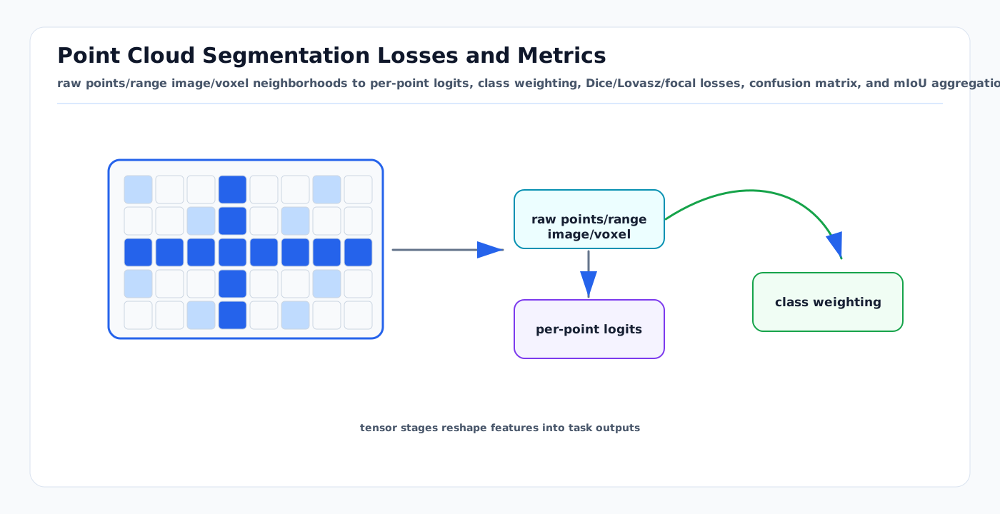
Visual: raw points/range image/voxel neighborhoods to per-point logits, class weighting, Dice/Lovasz/focal losses, confusion matrix, and mIoU aggregation.
Point cloud segmentation assigns a class label to each point, voxel, range-image pixel, or fused map element. The core difficulty is not just 3D geometry. It is the mismatch between training tensors, irregular sensor sampling, severe class imbalance, ignored labels, and metrics such as mean intersection over union that care about rare classes as much as common ones.
Related Docs
- PointPillars: First Principles
- Sparse Attention for 3D Perception
- Logistic, Softmax, and Cross Entropy
- Detection Theory: ROC, PR, and Operating Points
- LiDAR Semantic Segmentation — methods overview
- Aggregated-Map Semantic Segmentation — §6.5 losses and §13 evaluation
- 3D Segmentation Training Paradigms — map-derived label eligibility
Why It Matters
| Choice | Effect | Risk if wrong |
|---|---|---|
| Representation | Raw points, range image, voxels, pillars, or BEV. | Metric hides projection holes or voxel aliasing. |
| Sampling | Selects neighborhoods and batch points. | Rare classes disappear from gradients. |
| Loss | Defines per-point learning pressure. | Background dominates or small objects fragment. |
| Ignore policy | Excludes unlabeled or ambiguous points. | Model is punished for label uncertainty. |
| Metric | Summarizes confusion matrix. | High pixel/point accuracy with unsafe rare-class misses. |
Tensor Pipeline and Label Space
raw points (x, y, z, intensity, time)
  -> range image, voxel grid, pillar grid, sparse tensor, or point neighborhoods
  -> local feature aggregation
  -> per-point or per-cell logits
  -> projection back to original points if needed
Loss and metrics must be computed in the same label space. Three regimes:
Point-based (PTv3, PointNet++): Loss on raw points. No label-space mismatch; large batch sizes required for stable Lovász gradients.
Voxel-based (MinkUNet, Cylinder3D): Multiple points collapse to one voxel by majority-vote label. Thin-structure points in the minority of a voxel lose their label — implicit rare-class downsampling. Recommended voxel size for aggregated maps: 5–10 cm. Voxel labels are projected back to raw points at inference by nearest-neighbor lookup.
Range-view (RangeFormer, SalsaNext): Loss on the 2D range-image grid. Multiple 3D points project to the same pixel (many-to-one); kNN post-processing reassigns predictions to all corresponding 3D points. Gradients flow through 2D, not 3D geometry.
If the network predicts on voxels but the benchmark evaluates original points, the projection is part of model behavior and must be validated separately.
Pointwise Classification Losses
Softmax + Cross-Entropy
p_ic = exp(s_ic) / sum_k exp(s_ik)
L_CE = -(1/N) * sum_n log(y_n^{c*_n})
Gradient of CE w.r.t. logit z_c is (y_c - t_c). Well-classified easy points contribute non-trivially because log decays slowly, so dominant classes (ground, pavement) swamp gradients for rare classes (personnel, aircraft stairs). CE alone is insufficient when class imbalance exceeds ~20:1.
Weighted Cross-Entropy and the Three Weighting Schemes
L_WCE = -(1/N) * sum_n sum_c w_c * t_n^c * log(y_n^c)a) Inverse frequency: w_c = 1 / f_c where f_c = count_c / N_total. Simple; can over-weight rare classes and cause gradient instability with noisy labels.
b) Inverse square-root frequency: w_c = 1 / sqrt(f_c). Softer; the standard choice in SemanticKITTI baselines.
c) Effective number of samples (Cui et al. CVPR 2019):
EN(n_c) = (1 - beta^{n_c}) / (1 - beta)
w_c = (1 - beta) / (1 - beta^{n_c})   [normalize so sum = C]
Intuition: marginal benefit of a new sample diminishes as the class grows (data overlap). beta = 0 → uniform; beta → 1 → inverse frequency. beta = 0.9999 is typical for very long-tailed datasets. Theoretically grounded; preferred for extreme imbalance.
All static weight schemes are set before training and cannot adapt to within-batch difficulty; validate gradient magnitudes per class after switching.
Label Smoothing and OHEM
Label Smoothing: t_smooth^c = (1-eps)*t^c + eps/C (eps = 0.1 standard). Penalizes overconfident logit gaps; consistently improves ECE. Calibration regularizer, not a class-imbalance fix. SVLS applies a Gaussian kernel to one-hot GT so boundary points receive distributed labels. Margin-Based LS (Murugesan et al. 2022) enforces a logit-gap inequality constraint, achieving state-of-the-art calibration while maintaining discriminative accuracy.
OHEM: after a forward pass, sort per-point CE losses descending; backpropagate through only the top-k% hardest points (k = 10–25%). Focuses gradient budget on informative points but provides no class-rebalancing. Stratified OHEM samples proportionally across loss ranges. Combine with class weights or Lovász.
Focal Loss
Lin et al. ICCV 2017:
FL(p_t) = - alpha_t * (1 - p_t)^gamma * log(p_t)
  p_t = p (correct class) or 1-p (wrong class)
  gamma = 2 recommended; at gamma=0, alpha_t=1: FL reduces to CE
(1 - p_t)^gamma suppresses gradient from easy points; p_t > 0.8 contributes ~(0.2)^2 = 4% of normal weight. Helps: few-class strong foreground/background imbalance (aircraft service vehicles vs. tarmac); adaptive vs. static WCE. Hurts: highly multi-class settings — a single gamma does not adapt per class; noisy rare-class labels are amplified. Standard focal loss worsens ECE (gamma exponent causes systematic under-confidence); apply temperature scaling post-hoc. Dual Focal Loss applies class-specific modulation factors to address this.
Region and Overlap Losses
Dice Loss
L_Dice = 1 - (1/C) * sum_c [2 * sum_n t_n^c * y_n^c] / [sum_n (t_n^c + y_n^c)]Normalizes by total foreground mass; small classes (aircraft nose gear, apron stand markers) get amplified gradients — natural class-size invariance unlike CE. Limitation: weights FP and FN equally. Use Tversky when FN are more costly.
Soft-Jaccard / Soft-IoU
L_IoU = 1 - (1/C) * sum_c [sum_n t_n^c * y_n^c]
                           / [sum_n (t_n^c + y_n^c - t_n^c * y_n^c)]
More demanding than Dice (IoU = Dice / (2 - Dice)). This is a differentiable approximation; Lovász-Softmax is the principled convex surrogate.
Tversky Loss (Salehi et al. 2017)
TI_c = [sum_n t_n^c * y_n^c]
     / [sum_n t_n^c * y_n^c + alpha * FN_terms + beta * FP_terms]
L_Tversky = 1 - (1/C) * sum_c TI_c
  alpha=beta=0.5 -> Dice; alpha=beta=1.0 -> Jaccard
For airside maps where missed structures (FN) matter more than false alarms, set alpha > 0.5 (e.g., alpha = 0.7, beta = 0.3).
Focal Tversky Loss (Abraham & Khan 2019): L_FT = sum_c (L_T^c)^{1/gamma}. Applies a focal exponent to per-class Tversky loss; hard/rare classes contribute more. Warning: near convergence, well-classified classes may have near-zero gradients — monitor per-class training curves.
Generalized Dice Loss (Sudre et al. MICCAI 2017)
GDL = 1 - 2 * [sum_l w_l * sum_n r_ln * p_ln] / [sum_l w_l * sum_n (r_ln + p_ln)]
GDL_v variant: w_l = 1 / (sum_n r_ln)^2
Each class weighted by inverse square of its point count. A class with 10x fewer points gets ~100x higher weight, automatically correcting the size-Dice correlation without manual tuning. Validated down to imbalance ratios of 0.002, substantially outperforming WCE and per-class Dice.
Lovász-Softmax
Derivation — Submodular Jaccard and the Lovász Extension
The IoU/Jaccard score is discrete and non-differentiable. The Jaccard loss Delta_J_c = 1 - J_c is submodular:
Delta(A) + Delta(B) >= Delta(A union B) + Delta(A intersect B)Submodular functions have a canonical convex continuous relaxation — the Lovász extension — which is the basis for Lovász-Softmax (Berman et al. CVPR 2018).
The Lovász Extension
f_bar(m) = sum_{i=1}^{P} m_{pi_i} * g_i(m)

  m       = continuous error vector in [0,1]^P
  pi      = permutation sorting m decreasingly
  g_i(m)  = Delta({pi_1,...,pi_i}) - Delta({pi_1,...,pi_{i-1}})
             (marginal IoU loss as each sorted error is added)
The Lovász extension of a submodular function is convex and piecewise linear — an exact convex lower bound tight at binary vertices.
From Softmax to Errors
m_i(c) = 1 - f_i(c)   if c == c*_i  (true class)
m_i(c) = f_i(c)        otherwise     (wrong class)
The Loss and Algorithm
L_Lovász = (1/|C_present|) * sum_{c in C_present} Delta_J_bar_c(m(c))"Present classes" restriction: compute the mean only over classes present in the batch to approximate dataset-level mIoU. Algorithm: (1) compute error vector m(c); (2) sort decreasingly — O(P log P); (3) walk sorted errors, build g_i incrementally at O(1)/step; (4) dot product gives L_Lovász-c. Total: O(P log P) per class per batch.
Why not use Lovász alone: unstable gradients early in training (sorted permutation changes every iteration). CE provides the stable baseline. Lovász also does not handle class imbalance (equal weight per present class), so pair with WCE when imbalance is severe.
Boundary-Aware Losses
Boundary Loss (Kervadec et al. 2019): computes a distance metric on contours rather than region volumes — important when regional integrals are overwhelmed by dominant classes:
L_B = integral_Omega phi_G(q) * s(q) dq
  phi_G(q) = signed distance map of GT boundary (positive outside, negative inside)
  s(q)     = predicted soft probability
phi_G is pre-computed and fixed; L_B is linear in softmax outputs, making gradients straightforward. For airside LiDAR: aircraft edges, runway centerlines, taxiway markings, approach light poles are all thin in 3D. Boundary loss penalizes misplacement even when total misclassified point count is small.
Distance-Map CE (DMCE): L_DMCE = -sum_n (1+Phi_n) * log(t_n · y_n) where Phi_n is inverse distance to nearest boundary. Simpler; useful when signed distance maps are expensive to precompute at scale.
Active Boundary Loss (Wang et al. AAAI 2022): detects predicted boundaries via KL divergence of neighboring point predictions, then applies CE with directional guidance from GT boundaries. No explicit boundary labels required beyond segmentation labels.
Loss Combination and What Leading Methods Use
The Standard Recipe
L_total = L_CE (or L_WCE) + lambda * L_Lovász (or L_Dice)CE provides stable pointwise gradient; Lovász/Dice aligns training with mIoU. Normalize both to comparable scales before setting lambda — CE values are ~0.5–2.0 nats; Lovász is bounded in [0, 1]. Starting point: lambda = 1.0. Some implementations ramp lambda up during training (CE-dominated early, then increasing Lovász weight) for stability.
Release-State-Aware Map Objective
Aggregated-map labels are not just semantic labels. A map-derived training point also carries a hygiene or release-state label such as permanent_static, dynamic_residual, movable_static, static_transient, fod_candidate, artifact, or unknown_review. The loss must therefore answer two questions: what class is the point, and is that point eligible to supervise permanent map truth?
L_total =
  L_semantic(mask_semantic_positive)
  + alpha * L_release_state(mask_release_labeled)
  + beta  * L_hard_negative(mask_dynamic_or_transient)
  + gamma * L_calibration(mask_exportable)

mask_semantic_positive =
  release_state == permanent_static
  and source_map_acceptance == pass
  and confidence >= tau_semantic
  and split_id not in validation/test
The semantic head predicts the controlled class taxonomy. The release-state head predicts or audits permanence and hygiene. The two heads may share the same backbone, but their targets must not be collapsed into one class ID. A correctly classified stationary person is still a negative for the permanent map; a correctly classified FOD-like point may be a hazard-review target rather than background; an artifact-like cluster should not teach the model that thin wires or poles are noise unless source-quality evidence proves it.
| Release state | Semantic loss treatment | Auxiliary target | Evaluation guard |
|---|---|---|---|
permanent_static | Positive class target | Optional permanence-positive label | Per-class IoU, boundary F1, calibration |
dynamic_residual | Ignore for static semantics or hard negative near permanent classes | Dynamic-removal / MOS target | Residual-dynamic rate, false-deletion rate |
movable_static | Ignore for permanent-map positives unless consumer requests context | Movable-context or soft-occupancy target | False-permanent rate, TTL expiry accuracy |
static_transient | Hard negative for permanent-map training | Transient-object target | Stationary-person / temporary-asset leakage |
fod_candidate | Active-learning target after review, otherwise ignore | Hazard-candidate target | FOD exclusion and reviewer disposition |
artifact | Ignore or artifact auxiliary target | Artifact/noise target | Artifact-vs-thin-structure confusion |
unknown_review | No supervised positive | Unknown / abstention target | Review yield and promotion/demotion outcome |
This is a multi-task objective, not a larger semantic taxonomy. Adding dynamic_residual as a semantic class would let the model optimize mIoU while hiding the release decision. Keeping release state as a separate head or mask lets the same point cloud support three products: a publishable semantic layer, a rejected-evidence layer, and a training-export manifest with clean loss masks.
What State-of-the-Art Models Use
| Model | Loss Configuration | Representation |
|---|---|---|
| PTv3 (CVPR 2024) | CE (1) + Lovász (1), AdamW, cosine LR | Point-based |
| Cylinder3D (CVPR 2021) | WCE + Lovász-Softmax | Cylindrical voxel |
| MinkUNet | WCE + Lovász-Softmax (Pointcept) | Sparse voxel |
| SPVCNN | CE + Lovász (semseg-cac-v1m1-1-spunet-lovász config) | Hybrid |
| RangeFormer (ICCV 2023) | WCE + Lovász | Range-view |
| TORNADO-Net | WCE + Lovász + Total Variation | Range-view |
Exact lambda values and weight schedules for Cylinder3D and RangeFormer could not be confirmed from public sources; consult official training configs.
Loss Quick-Reference
| Loss | Imbalance | IoU-Optimal | Calibration | Airside Notes |
|---|---|---|---|---|
| CE | No | No | Overconfident | Baseline; use with WCE |
| WCE (ISRF) | Yes | No | Moderate | Standard for SemanticKITTI |
| WCE (Effective N) | Yes — principled | No | Moderate | Better for extreme tail |
| Label Smoothing | Partial | No | Good | Combine with CE/WCE |
| Focal Loss | Adaptive | No | Often worse | gamma=2; caution with noise |
| GDL | Yes — auto | Partial | Neutral | Good for small 3D structures |
| Tversky | Yes (alpha/beta) | Partial | Neutral | FN-heavy: alpha > 0.5 |
| Lovász-Softmax | No | Yes | Neutral | Standard add-on to CE/WCE |
| Boundary Loss | No | No | Neutral | Critical for thin airside structures |
| WCE + Lovász | Yes | Yes | Moderate | Best single recipe for LiDAR |
Class Imbalance Beyond the Loss
Resampling: oversample voxels/crops centered on rare-class instances; weight which scans to draw by inverse rare-class frequency. In aggregated maps, apply voxel-grid or farthest-point subsampling to equalize spatial density before loss computation (near-field cm-level vs. far-field >1 m spacing).
Copy-Paste / Instance Augmentation: extract 3D instance point clouds (GSE, personnel, chocks) from a library and paste into new scenes with rotation, scaling, and noise augmentation. Handles infrequent natural occurrence of rare classes.
PolarMix (NeurIPS 2022): two operations in polar coordinates: (1) instance rotation-paste at multiple angles; (2) scan-level azimuth sector swap between two scans, preserving LiDAR density and occlusion structure. Gains: MinkUNet on SemanticKITTI +2.9% mIoU (65.0→67.9%); SPVCNN +1.3% (66.2→67.5%). Also achieves equivalent mIoU with only 75% of training data. Note: assumes single- scan structure; for aggregated maps use crop + density-normalized subsampling + instance copy-paste instead. DACB-PolarMix fixes the equal-probability limitation by scaling augmentation count per class underrepresentation.
LaserMix (CVPR 2023 Highlight): semi-supervised framework partitioning points by elevation inclination band and interleaving alternate bands from two scans. Consistency regularization on labeled and mixed scans; pseudo-labels filtered by confidence threshold. Reported 10.8% relative improvement over supervised-only baseline; competitive with 2–5× fewer labels on nuScenes and SemanticKITTI.
Evaluation Metrics
Confusion Matrix, IoU, and mIoU
C_ab = number of points with GT class a predicted as class b

TP_c = C_cc
FP_c = sum_{j!=c} C_jc    (predicted c but not c)
FN_c = sum_{j!=c} C_cj    (are c but not predicted c)

IoU_c = TP_c / (TP_c + FP_c + FN_c)
mIoU  = (1/C) * sum_c IoU_c
mIoU is a macro-average: each class contributes equally regardless of frequency. Exclude classes absent from both prediction and GT in a tile (treat as NaN, not 0) to avoid artificially inflating scores on sparse sets. Standard for all major 3D benchmarks (SemanticKITTI, nuScenes, Waymo, ScanNet) because it is decomposable per class and makes rare classes visible.
Micro-IoU = sum_c TP_c / sum_c (TP_c + FP_c + FN_c) pools across classes and is dominated by the most frequent; not the primary metric in 3D segmentation.
FWIoU, OA, mAcc, Precision/Recall/F1
FWIoU = sum_c [freq_c * IoU_c]   freq_c = (TP_c + FN_c) / total points
OA    = sum_c TP_c / N_total
Acc_c = TP_c / (TP_c + FN_c)
mAcc  = (1/C) * sum_c Acc_c
Precision_c = TP_c / (TP_c + FP_c)
F1_c  = 2 * Precision_c * Recall_c / (Precision_c + Recall_c)
FWIoU: weighted by class point fraction — captures total-map coverage quality but downweights rare safety-critical classes; secondary metric only. OA: dominated by majority class; easy to game. mAcc: ignores false positives; useful when recall matters more than precision. F1 >= IoU always (more conservative denominator); use IoU for 3D leaderboards.
Panoptic and 4D Metrics
Panoptic Quality (PQ = SQ × RQ), PQ†, LSTQ, MOS IoU
Kirillov et al. CVPR 2019. Match predicted segment p and GT g if IoU(p,g) > 0.5 (unique, unambiguous):
SQ_c = sum_{(p,g) in TP_c} IoU(p,g) / |TP_c|           [shape quality, in [0.5,1]]
RQ_c = |TP_c| / (|TP_c| + 0.5|FP_c| + 0.5|FN_c|)       [F1 for detection]
PQ_c = SQ_c * RQ_c                                        [penalizes both]
Benchmarks report PQth (things) and PQst (stuff). Airside: things = aircraft, GSE, vehicles, persons; stuff = pavement, markings, buildings, fencing.
PQ† (PQ-dagger): for stuff, uses full-class IoU instead of per-connected- component matching. Prevents over-penalizing correct but fragmented ground or pavement predictions common in LiDAR benchmarks.
LSTQ (Aygün et al. CVPR 2021): LSTQ = sqrt(S_cls * S_assoc). S_cls = mIoU over the full 4D point set; S_assoc = temporal instance consistency (association IoU in space-time; objects < 50 points excluded). Geometric mean enforces both components must be strong. Mandatory for multi-scan or sequential LiDAR.
MOS IoU: binary moving/static; primary scalar is IoU_moving. mIoU_obj averages IoU across instances rather than points, correcting bias toward large nearby objects.
Boundary, Calibration, and Robustness Metrics
Boundary IoU, Calibration, Robustness, and OOD Metrics
Boundary IoU (Cheng et al. 2021):BIoU_c = |delta_P_c(d) intersect delta_G_c(d)| / |delta_P_c(d) union delta_G_c(d)| Restricts evaluation to a band of width d (0.1–0.5 m in 3D) around segment boundaries. Penalizes boundary misplacement; interior errors are downweighted. Critical for thin airside structures: runway markings, approach lights, jet bridges, fencing.
Calibration metrics:
ECE = sum_{m=1}^{M} (|B_m|/n) * |acc(B_m) - conf(B_m)|   [M=10 or 15 bins]
MCE = max_m |acc(B_m) - conf(B_m)|
BS  = (1/N) * sum_i sum_c (p_{i,c} - y_{i,c})^2
NLL = -(1/N) * sum_i log p_{i, y_i}
Reliability diagram: conf on x-axis, acc on y-axis; perfect calibration = y = x. Temperature scaling (post-hoc): p_c = softmax(logits / T)_c; T > 1 softens without changing argmax. Local Temperature Scaling learns a spatially varying T via a small CNN. Modern networks are systematically overconfident (Guo et al. 2017). Calibration is a safety property: overconfident wrong labels bypass uncertainty-gating in occupancy maps and planners, causing silent map errors.
Robustness (Robo3D / Kong et al. ICCV 2023): eight corruption types (Fog, Wet Ground, Snow, Motion Blur, Beam Missing, Crosstalk, Incomplete Echo, Cross- Sensor), three severities:
CE_i = sum_l [1-mIoU_{i,l}] / sum_l [1-mIoU_{i,l}^{baseline}]
mCE  = (1/8) * sum_i CE_i
mRR  = (1/8) * sum_i [sum_l mIoU_{i,l} / (3 * mIoU_clean)]
CE_i < 1: model degrades less than MinkUNet baseline. mCE is baseline-relative; not comparable across papers using different baselines. Airside: Fog/Wet Ground are primary apron risks; Beam Missing models occlusion by jet blast.
OOD and Uncertainty:
AUROC = integral TPR(t) d FPR(t)              [0.5 = chance]
AUPRC = integral Precision(t) d Recall(t)     [primary OOD metric]
FPR95 = FP/(FP+TN) at TPR = 0.95             [safety operating point]
AUSE  = integral [metric_model(f) - metric_oracle(f)] df
PAvPU = (AC + IU) / ALL   [accurate&certain + inaccurate&uncertain]
Exclude no-return voxels from OOD evaluation (structural, not anomalous). Lower AUSE = uncertainty better predicts actual errors.
Statistical Rigor and Reporting
- Hidden test servers: repeated submissions to SemanticKITTI/nuScenes/Waymo allow implicit test-set optimization; leaderboard rankings can diverge from true model quality as submission counts accumulate.
- Multi-seed variance: report mean ± std over ≥ 3 seeds (5 preferred). Use the same seed across ablation conditions. Typical variance: ±0.3–0.8% mIoU for large LiDAR models.
- Significance testing: Wilcoxon signed-rank or Friedman test preferred (segmentation score distributions are non-Gaussian); bootstrapped CIs also widely used. State: "A achieves X±Y mIoU vs. B at X'±Y', p < 0.05."
- Leaderboard hygiene: report which split all hyperparameters were tuned on; never pool validation and test for final reporting.
QA for Aggregated-Map Segmentation
Spatial Tile Splits — Not Random Point Splits
Spatial autocorrelation in LiDAR means a random point split leaks information (adjacent points in the same scan appear in both sets). Required protocol:
- Split the map into spatial tiles (e.g., 50 m × 50 m for an apron) before any annotation or training.
- Reserve ≥ 20% of non-contiguous tiles as a held-out test set.
- Evaluate mIoU, per-class IoU, coverage, and calibration on held-out tiles only.
- For cross-site generalization, use tiles from a second airport as the test.
Coverage Metric
Coverage = |{p : max_c P(c|p) >= tau}| / |P_total|tau = 0.8–0.9. Reports the fraction of map points labeled with sufficient confidence. A minimum coverage target (e.g., ≥ 95% at tau ≥ 0.8) is a deployment gate, not just a reporting number. Stratify by class: a map may be 99% covered for ground but 70% for rare classes such as GSE equipment.
Cross-Site Delta-mIoU
delta_mIoU_cross = mIoU_source_test - mIoU_target_zero_shotQuantifies domain shift from sensor model, mounting geometry, point density, and class distribution differences. Report per-class IoU drop to identify the most domain-sensitive classes. Fine-tuned delta (with N labeled target-site tiles) quantifies adaptation cost.
Error Decomposition, Stratified Evaluation, and Baseline Cross-Check
MDE (Mean Distance Error):
MDE_c = (1/|misclassified as c|) * sum_i min_{j: GT=c} ||p_i - p_j||
mMDE  = (1/C) * sum_c MDE_c
Low MDE = boundary errors (adjacent-class confusion). High MDE = whole-region confusion (taxiway labeled as runway at different location). Actionable split: boundary errors → resolution or post-processing; whole-region → training data gaps. Proportion of Distant Errors (rho_c): fraction of class-c errors exceeding a class-specific distance threshold; high rho_c = systematic confusion, not boundary slop.
Density stratification: bin map points by local density (points/m²) into Low/Medium/High; evaluate mIoU per bin. Models trained on dense scans fail on sparse distant regions (approach light poles, apron edges). Intensity stratification: high-intensity (retroreflective markings) vs. low-intensity (asphalt, grass) bins to verify the model exploits the intensity channel.
Fine-grained hierarchical mIoU (arXiv 2407.21289): mIoU^I (instance-level, distributes FP by instance size) is the most appropriate primary metric for airside maps where small objects (personnel, cones, chocks) are safety-critical but contribute few points. Also: mIoU^D (dataset-level, dominant-class biased), mIoU^P (per-scan averaged), mIoU^C (category-ordered, frequency-bias reduced).
Classical heuristic baseline cross-check: compare against height thresholding
- RANSAC plane fitting + intensity-bin pavement marking rules. If the learned model does not achieve ≥ 3% mIoU gain on held-out tiles, the added complexity is unjustified — investigate whether the model learned sensor-make artifacts rather than generalizable geometric features.
Map-Hygiene Metrics for Removal and Quarantine
Aggregated-map segmentation is only valid if the map substrate is clean enough to label. Report semantic metrics together with map-hygiene metrics so a high mIoU score cannot hide dynamic residuals, false deletion, or transient-object leakage.
dynamic_residual_rate =
  points labeled dynamic-residual or no-class-possible / total map points

false_permanent_rate =
  transient GT points published in permanent layer / transient GT points

false_deletion_rate =
  permanent GT points removed or quarantined / permanent GT points

transient_leakage_rate =
  transient-layer points used for auto-label training / transient-layer points
For safety-critical map products, these rates should be stratified by class and zone. A low global false-permanent rate is not enough if gate zones, dock doors, pedestrian corridors, or FOD-critical pavement have higher leakage.
| Metric | What it catches | Why mIoU misses it |
|---|---|---|
| Dynamic residual rate | Ghost trails or motion smears left in the map | Residual points may be labeled as plausible nearby classes |
| False permanent rate | Stationary people, parked GSE, aircraft, pallets, or barriers baked into permanent map | Semantic class can be correct while permanence is wrong |
| False deletion rate | Poles, signs, kerbs, markings, drains, fences removed by aggressive cleaning | Deleted points are absent from the segmentation denominator unless explicitly audited |
| Transient leakage rate | Quarantined points reused as pseudo-label ground truth | Training data quality can degrade while map metrics still look acceptable |
| Review burden per area | Human QA cost in low-confidence or disagreement regions | Accuracy metrics do not measure operational cost |
The correct evaluation object is therefore a tuple:
(semantic labels, confidence, map layer, provenance, reviewer/gate decision)not just a per-point class ID. This tuple is the bridge between point-cloud segmentation metrics and the map-publication evidence expected by the aggregated-map pipeline.
Implementation Notes
- Apply ignore masks before both loss and metrics; unlabeled points must not become background.
- For map-derived labels, compute the semantic loss mask from release state, source-map acceptance, confidence, and split assignment before the first training step; never let transient, artifact, or review-only points default to background.
- Preserve original point indices through voxelization or range projection so metrics can be computed on the benchmark point set.
- Track class frequency before and after augmentation, sampling, and cropping.
- Evaluate range bands separately; far points are sparse and dominate missed- object risk.
- Separate static labels from moving labels if the dataset uses both.
- Calibrate logits before they feed mapping or planning.
- Keep a "void/unknown" policy explicit at the map boundary.
- For aggregated maps: implement per-point confidence scores or mean-aggregated logits for overlapping multi-scan regions with conflicting labels.
- Deep supervision: auxiliary heads at decoder scales with lambda_k ~ 0.4 for intermediate heads and 1.0 for the final head; improves gradient flow in deep U-Net architectures.
Failure Modes
| Symptom | Likely cause | Diagnostic |
|---|---|---|
| High accuracy, low mIoU. | Background or road dominates. | Inspect classwise IoU and confusion matrix. |
| Small objects vanish. | Sampling or loss ignores rare points. | Count rare-class points per batch. |
| Boundary shimmer. | Voxel/range projection loses detail. | Compare raw point labels with projected predictions. |
| Moving classes confused with static. | Temporal labels or aggregation policy mismatched. | Evaluate moving/static classes separately. |
| Map fusion becomes overconfident. | Softmax scores uncalibrated. | Reliability diagram per class and range band. |
| Lovász improves mIoU but hurts safety. | Rare class tradeoff hidden in mean. | Review per-class precision and recall. |
| mIoU inflated on validation, not test. | Random point split (autocorrelation leakage). | Switch to spatial tile splits; re-evaluate. |
| Cross-site performance collapses. | Model learned sensor-make or density artifacts. | Run classical heuristic baseline as sanity floor. |
| Dense near-field dominates loss. | Aggregated map density non-uniform. | Apply voxel-grid subsampling before loss. |
Sources
- Qi et al., PointNet: https://arxiv.org/abs/1612.00593
- Qi et al., PointNet++: https://arxiv.org/abs/1706.02413
- Behley et al., SemanticKITTI: https://arxiv.org/abs/1904.01416
- Berman, Triki, Blaschko, Lovász-Softmax (CVPR 2018): https://arxiv.org/abs/1705.08790
- Sudre et al., Generalised Dice (MICCAI 2017): https://arxiv.org/abs/1707.03237
- Lin et al., Focal Loss (ICCV 2017): https://arxiv.org/abs/1708.02002
- Hu et al., RandLA-Net: https://arxiv.org/abs/1911.11236
- Cortinhal et al., SalsaNext: https://arxiv.org/abs/2003.03653
- Cui et al., Class-Balanced Loss / Effective Number (CVPR 2019): https://arxiv.org/abs/1901.05555
- Abraham & Khan, Focal Tversky (2019): https://arxiv.org/abs/1810.07842
- Salehi et al., Tversky Loss (2017): https://arxiv.org/abs/1706.05721
- Kervadec et al., Boundary Loss (2019): https://arxiv.org/abs/1812.07032
- Wu et al., PTv3 (CVPR 2024): https://arxiv.org/abs/2312.10035
- Zhu et al., Cylinder3D (CVPR 2021): https://arxiv.org/abs/2008.01550
- Kong et al., RangeFormer (ICCV 2023): https://arxiv.org/abs/2303.05367
- Loss Functions in Semantic Segmentation Survey (arXiv 2312.05391): https://arxiv.org/html/2312.05391v1
- Xiao et al., PolarMix (NeurIPS 2022): https://openreview.net/pdf?id=wS23xAeKwSN
- Kong et al., LaserMix (CVPR 2023): https://arxiv.org/abs/2207.00026
- Murugesan et al., Margin-Based Label Smoothing (2022): https://arxiv.org/abs/2209.09641
- SVLS — Spatially Varying Label Smoothing: https://arxiv.org/pdf/2104.05788
- Local Temperature Scaling: https://arxiv.org/abs/2008.05105
- Mukhoti et al., Calibrating DNNs using Focal Loss (NeurIPS 2020): https://arxiv.org/abs/2002.09437
- Kirillov et al., Panoptic Segmentation (CVPR 2019): https://openaccess.thecvf.com/content_CVPR_2019/papers/Kirillov_Panoptic_Segmentation_CVPR_2019_paper.pdf
- Aygün et al., 4D Panoptic LiDAR Segmentation (CVPR 2021): https://www.researchgate.net/publication/355864674_4D_Panoptic_LiDAR_Segmentation
- Panoptic nuScenes: https://arxiv.org/pdf/2109.03805
- Cheng et al., Boundary IoU (2021): https://arxiv.org/abs/2103.16562
- Guo et al., On Calibration of Modern Neural Networks (2017): https://arxiv.org/pdf/1706.04599
- Calibration Survey 2023: https://arxiv.org/pdf/2308.01222
- Kong et al., Robo3D (ICCV 2023): https://arxiv.org/abs/2303.17597
- LiDAR OOD detection with epistemic uncertainty: https://arxiv.org/html/2510.08631
- Fine-Grained PC Metrics (arXiv 2407.21289): https://arxiv.org/html/2407.21289v1
- Spatially-Aware Aerial LiDAR Evaluation (arXiv 2603.22420): https://arxiv.org/html/2603.22420
- PQ† / Panoptic Tracking Survey (arXiv 2212.13445): https://arxiv.org/pdf/2212.13445
- DACB-PolarMix (PLOS ONE 2025): https://pmc.ncbi.nlm.nih.gov/articles/PMC11913263/
- Real3D-Aug: https://arxiv.org/pdf/2206.07634
- Uncertainty-Aware LiDAR Panoptic Seg: https://arxiv.org/pdf/2210.04472
- BEV Uncertainty Benchmark (arXiv 2405.20986): https://arxiv.org/html/2405.20986
- Statistical Tests for ML: https://www.nature.com/articles/s41598-024-56706-x
- SemanticKITTI benchmark tasks: https://semantic-kitti.org/tasks.html
- Pointcept codebase: https://github.com/pointcept/pointcept
- Cylinder3D GitHub: https://github.com/xinge008/Cylinder3D