Feed-Forward 3D Reconstruction and Splatting
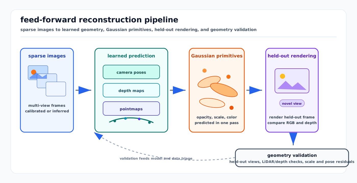
Visual: feed-forward reconstruction pipeline from sparse images through learned camera, depth, pointmap, and Gaussian prediction to held-out rendering and geometry validation.
Feed-forward 3D reconstruction spans the range from classical multi-view stereo (COLMAP, PatchMatch) through per-scene neural optimization (NeRF, 3DGS) to generalizable models (DUSt3R, VGGT, Splatt3R) that infer geometry in a single forward pass without per-scene training. This KB page covers first principles for all three tiers, with a focus on how each tier connects to the LiDAR-primary aggregated-map segmentation pipeline.
1. Related Docs
- Volume Rendering, Radiance Fields, and Gaussian Splatting — sibling KB page with shared NeRF/3DGS math
- Camera Projective Geometry, PnP, and Triangulation — DUSt3R/MASt3R use projective geometry at inference
- Point Cloud Representations and Voxelization: First Principles — the labeled aggregated map is the output product of both LiDAR pipelines and neural reconstruction
- Lie Groups SE(3), SO(3), Adjoints, and Jacobians — global alignment in DUSt3R optimizes over SE(3)
- Coordinate Frames, Projections, and SE(3) — camera frame conventions used throughout
- Neural Implicit SLAM and Differentiable Mapping
- Aggregated-Map Semantic Segmentation — §1.3 digital-twin / simulation assets output product; §4.2 LiDAR-camera fusion
- 3DGS Digital Twin — downstream consumer of 3DGS scenes produced by this pipeline
- Neural Scene Reconstruction — companion simulation overview
- Photoreal City-Scale 4D Reconstruction
- SLAM3R and VGGT Foundation SLAM
2. Why Reconstruction Matters for a LiDAR Segmenter
2.1 Why It Matters — at a Glance
| Connection | How it works | Why it is not optional |
|---|---|---|
| Output equivalence — labeled map IS labeled reconstruction | A segmented aggregated LiDAR map is geometry (from LiDAR) plus per-point semantic labels. A NeRF or 3DGS trained on labeled multi-view images produces the same artifact: a queryable 3D scene with per-point attributes. | Reconstruction pipelines and segmentation pipelines converge on the same data product. Methods transfer bidirectionally. |
| GS-SLAM / MASt3R-SLAM as camera-based map front-ends | Classical LiDAR-inertial odometry (LOAM, FAST-LIO2, LIO-SAM) builds the aggregated map incrementally. GS-SLAM, Gaussian Splatting SLAM, and MASt3R-SLAM are camera-derived dense map-building alternatives that produce the same geometry the segmenter labels. | Sensor-rich rigs (camera + LiDAR) can run both pipelines and fuse outputs. In camera-only segments of an airside environment, neural SLAM may be the only available front-end. |
| DUSt3R / VGGT as label-free 3D-feature pre-training | DUSt3R and VGGT pre-train large ViT backbones on massive RGB datasets to predict 3D geometry without calibration. Backbone weights encode geometrically grounded features. These can be used as a camera-branch feature extractor in LiDAR-camera fusion, providing a 3D geometric prior without any semantic labels. | Self-supervised 3D feature pre-training cuts label cost. VGGT demonstrated backbone transfer to non-rigid point tracking and novel-view synthesis; analogous transfer to 3D segmentation is an active research direction. |
| Digital-twin output | A photorealistic metrically accurate 3DGS digital twin of an airside apron is the output of reconstruction. It feeds simulation, synthetic data generation, and visual inspection. | Simulation assets (30-autonomy-stack/simulation/3dgs-digital-twin.md) are the downstream consumer. |
2.2 Three Concrete Coupling Points
(a) Labeled map = labeled reconstruction. Labeling methods from computer vision — open-vocabulary segmentation on rendered views, segment-and-lift, Feature-3DGS, LangSplat — can produce labels for 3DGS and NeRF scenes. A 3DGS scene with semantic SH or feature Gaussians is directly comparable in information content to a semantically labeled point cloud. The aggregated map can be rendered back to camera views for consistency checking or photometric augmentation.
(b) Reconstruction-based mapping as an alternative front-end. The following camera-based neural SLAM systems produce geometrically comparable dense maps alongside or instead of LIO:
| System | Base | FPS | Notes |
|---|---|---|---|
| NeRF-SLAM (arXiv:2210.13641) | NeRF | <1 | Dense but slow; offline use |
| GS-SLAM (CVPR 2024) | 3DGS | ~10 | Real-time potential |
| Gaussian Splatting SLAM (arXiv:2312.06741) | 3DGS | ~10 | Competitive tracking accuracy |
| MASt3R-SLAM (CVPR 2025 Highlight) | DUSt3R/MASt3R | 15 | No calibration needed; dense geometry |
| SGS-SLAM | Semantic 3DGS | ~5 | Directly outputs semantic map |
For an airside LiDAR rig, camera-derived dense SLAM can fill gaps in LiDAR coverage (glass walls, reflective markings) and provide appearance-rich geometry for simulation rendering.
(c) Label-free 3D feature pre-training. DUSt3R and VGGT produce geometrically grounded ViT features trained on massive unlabeled RGB datasets. Used as an image backbone in LiDAR-camera fusion — replacing, for example, a DINOv2 backbone with a DUSt3R-pretrained ViT — they provide a stronger geometric prior than pure photometric pre-training. In LiDAR-sparse scenarios (e.g., airside terminal interior), DUSt3R/VGGT can bootstrap a metric 3D map from available cameras alone.
3. Classical Multi-View Stereo (MVS)
3.1 Pipeline
Images
  -> Feature extraction  (SIFT, SuperPoint, LoFTR)
  -> Feature matching + outlier rejection  (RANSAC on fundamental matrix)
  -> Sparse SfM: triangulate 3D points, recover camera poses  (COLMAP)
  -> Dense MVS: per-pixel depth from photometric consistency  (PatchMatch)
  -> Depth-map fusion: merge per-image depthmaps into a dense point cloud
  -> Surface reconstruction: screened Poisson / NeuS -> mesh
COLMAP (Schonberger & Frahm, CVPR 2016; Schonberger et al., ECCV 2016) is the canonical open-source implementation of both SfM and PatchMatch MVS and remains the de-facto baseline for reconstruction benchmarks.
3.2 PatchMatch MVS
PatchMatch propagates depth and surface-normal hypotheses across neighboring pixels. Each pixel's depth is refined by checking photometric consistency across multiple source images. COLMAP's MVS stage uses PatchMatch as its core algorithm. PatchmatchNet (arXiv:2012.01411) is a learned variant. The key computational cost is the per-pixel multi-view comparison; GPU parallelism makes it tractable for moderate image counts.
3.3 Benchmarks
- Tanks and Temples (Knapitsch et al., SIGGRAPH 2017): outdoor and indoor scenes evaluated by F-score at precision/recall thresholds against ground-truth point clouds. URL: https://www.tanksandtemples.org/
- ETH3D (Schops et al., CVPR 2017): high-resolution multi-scale; F-score at 2 cm threshold. COLMAP scores approximately 73% F1 vs. state-of-the-art approximately 83% F1 on the ETH3D test split.
- DTU (Aanaes et al., IJCV 2016): controlled indoor; evaluated by Chamfer distance.
3.4 Limitations
MVS requires textured surfaces (untextured planar regions fail), controlled illumination, and overlapping views. Bundle adjustment complexity scales poorly with image count (O(n^2) or worse without sparsity tricks). Processing a large airside apron survey with thousands of images takes hours. These limitations are precisely the gap that feed-forward methods target.
4. Neural Radiance Fields (NeRF)
Paper: Mildenhall et al., "NeRF: Representing Scenes as Neural Radiance Fields for View Synthesis," ECCV 2020. URL: https://arxiv.org/abs/2003.08934
4.1 Representation
A NeRF represents a scene as a continuous volumetric field:
F_theta: (x, y, z, theta_view, phi_view) -> (sigma, r, g, b)where (x, y, z) is a 3D position, (theta_view, phi_view) is the viewing direction, sigma is volume density (opacity per unit length), and (r, g, b) is the view-dependent emitted color. The MLP F_theta has approximately 8 fully-connected layers of width 256, with a skip connection at layer 4.
4.2 Positional Encoding
Raw coordinates are too smooth for the MLP to represent high-frequency geometry and appearance. Mildenhall et al. apply Fourier feature lifting:
gamma(p) = [ sin(2^0 * pi * p),  cos(2^0 * pi * p),
             sin(2^1 * pi * p),  cos(2^1 * pi * p),
             ...
             sin(2^(L-1) * pi * p),  cos(2^(L-1) * pi * p) ]
L = 10 for position, L = 4 for viewing direction. This maps each scalar p in R^1 to R^(2L) and concatenates across the x, y, z, and direction dimensions.
4.3 Volume Rendering Integral
A camera ray r(t) = o + t * d is cast through the scene. The expected color along the ray is the continuous integral:
C(r) = integral_{t_near}^{t_far}  T(t) * sigma(r(t)) * c(r(t), d) dt

where the transmittance (probability of a photon reaching t unabsorbed):

T(t) = exp( -integral_{t_near}^{t}  sigma(r(s)) ds )
Discrete approximation with N stratified samples at positions t_1 < t_2 < ... < t_N, interval widths delta_i = t_{i+1} - t_i:
C_hat(r) = sum_{i=1}^{N}  T_i * alpha_i * c_i

where:
  alpha_i = 1 - exp(-sigma_i * delta_i)     [opacity of segment i]
  T_i     = prod_{j=1}^{i-1} (1 - alpha_j) [accumulated transmittance]
This is identical in form to classical alpha-compositing of sorted semi-transparent layers — a fact 3DGS exploits explicitly in its rasterizer.
4.4 Hierarchical Sampling
Two MLPs are used: a coarse network (N_c = 64 uniform stratified samples per ray) and a fine network (N_f = 128 additional samples, importance-sampled from the coarse density distribution). Both contribute to the training loss; the fine network is used for final rendering.
4.5 Training
Loss = mean squared photometric error between rendered and observed pixel colors, over a batch of 4096 randomly sampled rays. Training runs approximately 200k iterations, requiring 1-2 days on a V100 GPU for a single scene.
4.6 Speed Limitations
Vanilla NeRF requires hundreds of MLP evaluations per ray per frame. Rendering an 800x800 image takes approximately 30 seconds. Training requires hours to days. These limitations motivated the acceleration methods in Section 5.
5. NeRF Accelerations
5.1 Instant-NGP
Paper: Muller et al., "Instant Neural Graphics Primitives with a Multiresolution Hash Encoding," SIGGRAPH 2022. URL: https://arxiv.org/abs/2201.05989 Code: https://github.com/NVlabs/instant-ngp
Key idea: replace positional encoding with a learnable multiresolution hash table. For each resolution level l in {1,...,L} (L = 16 typical), the 3D position is hashed to a table of T feature vectors (T up to 2^24). Features from all levels are concatenated and passed to a tiny MLP (2 hidden layers, width 64). Hash collisions across levels cancel out via the MLP.
Speed: Training NeRF in approximately 5-10 seconds on a single GPU — a 1000x speedup over vanilla NeRF. Interactive rendering at approximately 60 FPS. Implemented via fully-fused CUDA kernels to minimize memory bandwidth.
5.2 Plenoxels
Paper: Fridovich-Keil et al., "Plenoxels: Radiance Fields without Neural Networks," CVPR 2022.
Key idea: replace the MLP entirely with a sparse voxel grid storing spherical harmonic (SH) coefficients per voxel. Volume rendering uses trilinear interpolation of grid values. No neural network at inference. Trains in approximately 10 minutes (approximately 100x faster than vanilla NeRF). Rendering is fast but quality lags Instant-NGP on fine details.
5.3 TensoRF
Paper: Chen et al., "TensoRF: Tensorial Radiance Fields," ECCV 2022. URL: https://apchenstu.github.io/TensoRF/
Key idea: decompose the 4D radiance-field tensor (3D space x feature channels) into a sum of vector-matrix outer products (VM decomposition) or CP decomposition. This reduces memory from O(n^3) to O(n^2) for VM decomposition or O(n) for CP decomposition. Competitive quality, standard PyTorch — no custom CUDA kernels required. Trains in approximately 30 minutes.
5.4 Acceleration Trade-off Summary
| Method | Training time | Rendering FPS | Memory | Quality |
|---|---|---|---|---|
| Vanilla NeRF | ~1-2 days | ~0.03 | ~1 GB | Very high |
| Plenoxels | ~10 min | ~15 | ~2 GB | Good |
| TensoRF | ~30 min | ~5 | ~0.5 GB | High |
| Instant-NGP | ~5-10 sec | ~60 | ~0.1 GB | High |
| 3DGS | ~30-60 min | 100+ | ~1 GB | Very high |
3DGS (Section 6) effectively superseded NeRF acceleration methods for real-time rendering use cases, while Instant-NGP remains valuable for rapid scene reconstruction in offline pipelines.
6. 3D Gaussian Splatting (3DGS)
Paper: Kerbl, Kopanas, Leimkuhler, Drettakis — "3D Gaussian Splatting for Real-Time Radiance Field Rendering," SIGGRAPH 2023. URL: https://repo-sam.inria.fr/fungraph/3d-gaussian-splatting/
6.1 Representation
A scene is modeled as an unordered set of N anisotropic 3D Gaussians. Each Gaussian i has:
mu_i    in R^3         : 3D mean (center position)
Sigma_i in R^(3x3)     : 3D covariance (positive semi-definite)
alpha_i in [0, 1]      : opacity
c_i     (SH coefficients): view-dependent color, degree-3 SH -> 48 scalars
The covariance is factored as:
Sigma = R * S * S^T * R^Twhere R is a rotation matrix (stored as unit quaternion q) and S = diag(s_x, s_y, s_z) is a diagonal scale matrix. This factorization guarantees positive semi-definiteness throughout gradient-based optimization.
The Gaussian density at a 3D point x:
G_i(x) = exp( -0.5 * (x - mu_i)^T * Sigma_i^{-1} * (x - mu_i) )6.2 EWA Projection from 3D to 2D
To rasterize, each 3D Gaussian is projected to an image-plane 2D Gaussian using the EWA (Elliptical Weighted Average) framework (Zwicker et al., TVCG 2002):
Sigma'_i = J * W * Sigma_i * W^T * J^Twhere:
- W in R^(3x3) is the viewing transformation (world-to-camera rotation)
- J in R^(2x3) is the Jacobian of the perspective projection evaluated at mu_i
The projected 2D mean mu'_i is the standard perspective projection of mu_i. The resulting 2D Gaussian is:
G'_i(x) = exp( -0.5 * (x - mu'_i)^T * Sigma'_i^{-1} * (x - mu'_i) )J is a first-order local approximation of the nonlinear projection, so EWA projection is exact only for small-footprint Gaussians. In practice this approximation is sufficient.
See also: Camera Projective Geometry, PnP, and Triangulation for the full projection chain and Jacobian derivation.
6.3 Tile-Based Differentiable Rasterizer
Gaussians are sorted by depth. The image is partitioned into 16x16 tiles. Per tile, visible Gaussians are alpha-composited front-to-back:
I(pixel) = sum_{k=1}^{K}  c_k * alpha_k * T_k

where:
  alpha_k  = G'_k(pixel) * opacity_k       [Gaussian footprint times stored opacity]
  T_k      = prod_{j < k} (1 - alpha_j)    [accumulated transmittance]
The rasterizer is GPU-implemented using CUDA tile sorting. Forward rendering achieves 100-160 FPS at 1080p on an NVIDIA RTX 3090. The backward pass for gradient-based optimization uses a custom reverse-mode pass that reads the sorted tile lists.
6.4 Adaptive Density Control
Training alternates gradient descent on (mu, q, s, alpha, SH) with density control every N iterations:
- Cloning: Gaussians in under-reconstructed regions (large positional gradient magnitude) are cloned and shifted to cover the gap.
- Splitting: Oversized Gaussians (large scale relative to scene extent) are split into two smaller Gaussians sampled from their distribution.
- Pruning: Gaussians with alpha below a threshold or that grow excessively large are removed.
The scene is initialized from a sparse SfM point cloud (COLMAP). Gaussians start with means at SfM points and small isotropic covariances.
6.5 Training Details
Loss:     L = (1 - lambda) * L1  +  lambda * L_DSSIM   (lambda = 0.2)
Training: ~30-60 minutes on NVIDIA RTX 3090 for a typical scene
Storage:  100-500 MB of Gaussian parameters (uncompressed)
6.6 Comparison to NeRF
| Aspect | NeRF (vanilla) | Instant-NGP | 3DGS |
|---|---|---|---|
| Representation | Implicit MLP | Hash grid | Explicit Gaussians |
| Rendering | Ray marching | Ray marching | Splatting / rasterization |
| Train time | ~2 days | ~10 sec | ~45 min |
| Render FPS | 0.03 | 60 | 100-160 |
| Editability | Very hard | Hard | Easy (explicit primitives) |
| Surface geometry | Implicit | Implicit | Implicit (extractable via 2DGS) |
7. 3DGS Variants
7.1 Mip-Splatting (CVPR 2024)
Paper: Yu et al., "Mip-Splatting: Alias-Free 3D Gaussian Splatting," CVPR 2024. URL: https://niujinshuchong.github.io/mip-splatting/
Addresses aliasing at different zoom levels. Replaces the standard 3D Gaussian with a 3D smoothing filter applied before projection, and uses a 2D Mip filter during rasterization. Result: consistent quality across training and rendering resolutions. Now adopted as a standard improvement in downstream 3DGS systems.
7.2 2D Gaussian Splatting (2DGS, SIGGRAPH 2024)
Paper: Huang et al., "2D Gaussian Splatting for Geometrically Accurate Radiance Fields," SIGGRAPH 2024. URL: https://surfsplatting.github.io/ GitHub: https://github.com/hbb1/2d-gaussian-splatting
Replaces 3D Gaussians with 2D oriented disks (flat Gaussians with one scale dimension near zero), forcing the representation to align with scene surfaces. Enables accurate surface normal estimation and clean mesh extraction from the splats. Critical for use cases that need geometric output — digital-twin geometry, structural inspection, clearance checks — rather than only photometric rendering.
7.3 4D Gaussian Splatting
Paper: Wu et al., "4D Gaussian Splatting for Real-Time Dynamic Scene Rendering," arXiv:2310.08528.
Adds a temporal dimension: each Gaussian has a time-varying mean and covariance modeled via 4D neural voxels. Achieves 82 FPS at 800x800 on RTX 3090 for dynamic scenes. Relevant for airside scenes with moving aircraft, vehicles, and ground crews where static 3DGS would bake motion artifacts.
7.4 Scaffold-GS (CVPR 2024 Highlight)
Paper: Lu et al., "Scaffold-GS: Structured 3D Gaussians for View-Adaptive Rendering," CVPR 2024. arXiv: https://arxiv.org/abs/2312.00109 URL: https://city-super.github.io/scaffold-gs/
Addresses the redundancy problem in vanilla 3DGS: too many Gaussians ignoring scene structure. Key idea: sparse anchor points (from SfM) each tether a set of neural Gaussians whose attributes (position offset, opacity, color) are predicted on-the-fly by a small MLP conditioned on anchor feature and viewing direction+distance. Anchor growing and pruning is based on neural Gaussian importance scores. Result: fewer primitives, faster convergence, and better quality on textureless regions.
7.5 Gaussian Splatting SLAM (CVPR 2024)
Paper: Matsuki et al., "Gaussian Splatting SLAM," arXiv:2312.06741, CVPR 2024. GS-SLAM: Yan et al., "GS-SLAM: Dense Visual SLAM with 3D Gaussian Splatting," CVPR 2024. URL: https://gs-slam.github.io/
Integrates 3D Gaussians as the live scene map in a real-time dense SLAM system. The differentiable rasterizer provides 100x faster rendering than NeRF-SLAM, enabling real-time tracking. Adaptive Gaussian expansion adds new Gaussians for newly observed geometry; old Gaussians are pruned. Tracking uses a joint photometric and depth loss against the current Gaussian map render.
8. Feed-Forward and Generalizable Reconstruction
The fundamental limitation of NeRF and 3DGS is per-scene optimization: each new scene requires hours of training. Feed-forward models learn scene priors from large datasets and reconstruct a new scene in a single forward pass (seconds or milliseconds) with no test-time optimization.
8.1 DUSt3R (CVPR 2024)
Paper: Wang, Leroy, Cabon, Chidlovskii, Revaud — "DUSt3R: Geometric 3D Vision Made Easy," CVPR 2024. CVF: https://openaccess.thecvf.com/content/CVPR2024/html/Wang_DUSt3R_Geometric_3D_Vision_Made_Easy_CVPR_2024_paper.html Project: https://europe.naverlabs.com/research/publications/dust3r-geometric-3d-vision-made-easy/
Pointmap formulation. Given an image pair (I^1, I^2), a pointmap X^{v,1} in R^{H x W x 3} assigns a 3D point in the coordinate frame of view v to every pixel of image 1. DUSt3R predicts four pointmaps:
- X^{1,1}: image 1 pixels in frame 1 (reference frame)
- X^{2,1}: image 1 pixels in frame 2
- X^{1,2}: image 2 pixels in frame 1
- X^{2,2}: image 2 pixels in frame 2 (reference frame)
Architecture. ViT-Large encoder with shared weights for both images. Two CroCo-style cross-attention decoder streams (one per image) that exchange information about the pair. Each decoder head regresses the pointmap and a confidence map C^v in R^{H x W x 1}.
Confidence-weighted loss:
L = sum over pixels p:
      C^v(p) * || X^v_pred(p) - X^v_gt(p) ||_2  -  alpha * log(C^v(p))
The confidence term down-weights ambiguous pixels (sky, reflective surfaces) and up-weights reliable ones. This is critical for outdoor scenes with large uniform regions.
Global alignment for N > 2 images. Pairwise pointmaps are predicted for all image pairs in a graph, then globally aligned:
argmin_{T_i in SE(3), s}  sum_{(i,j) in edges}
    sum_p  C^{i,j}(p) * || T_i * X^{i,j}(p) - s * X^{ref}(p) ||^2
using a differentiable optimizer (gradient descent on SE(3); see Lie Groups SE(3), SO(3), Adjoints, and Jacobians).
Output. 3D point cloud + camera poses + camera intrinsics — all from uncalibrated, unordered images in a single forward pass plus global alignment. Sets new state-of-the-art on monocular/multi-view depth estimation and relative pose estimation at CVPR 2024.
Implication for LiDAR pipelines. DUSt3R's ViT backbone encodes geometrically grounded features without any semantic supervision labels. These weights can serve as the image-branch feature extractor in LiDAR-camera fusion networks, providing a label-free 3D geometric prior.
8.2 MASt3R (ECCV 2024) and MASt3R-SLAM (CVPR 2025 Highlight)
Paper (MASt3R): Leroy et al., "Grounding Image Matching in 3D with MASt3R," ECCV 2024. URL: https://dl.acm.org/doi/10.1007/978-3-031-73220-1_5
Paper (MASt3R-SLAM): Edexheim et al., arXiv:2412.12392, CVPR 2025 Highlight. URL: https://arxiv.org/abs/2412.12392 / https://edexheim.github.io/mast3r-slam/
MASt3R augments DUSt3R with a dense matching head that outputs local feature maps alongside the pointmaps. A fast reciprocal matching scheme accelerates correspondence finding with theoretical guarantees, enabling scaling from 2 images to hundreds.
MASt3R-SLAM is a real-time monocular dense SLAM system built on MASt3R:
- No fixed camera model assumed (handles unknown or variable intrinsics)
- Efficient pointmap matching for camera tracking, local map fusion, loop closure
- Second-order global optimization for pose graph consistency
- 15 FPS real-time operation producing globally consistent poses + dense geometry
- Robust on in-the-wild video (no IMU, no calibration target required)
Comparison to classical LIO. MASt3R-SLAM is camera-only; it does not fuse IMU or LiDAR. For airside deployments with both camera and LiDAR, MASt3R-SLAM provides a camera-derived dense geometry stream that can be fused with LIO poses for robustness. Its advantage is dense geometry (not just sparse keypoints); its disadvantage is metric scale uncertainty without depth supervision.
8.3 VGGT (CVPR 2025 Best Paper)
Paper: Wang, Chen, Karaev, Vedaldi, Rupprecht, Novotny — "VGGT: Visual Geometry Grounded Transformer," CVPR 2025. arXiv: https://arxiv.org/abs/2503.11651 Code (Meta): https://github.com/facebookresearch/vggt Project: https://vgg-t.github.io/
VGGT is a feed-forward transformer that, given 1 to hundreds of input images, predicts all 3D attributes simultaneously in a single forward pass:
Input:   N RGB images (variable N, no calibration required)
Output:  camera intrinsics
         camera extrinsics (poses)
         per-image depth maps
         per-image pointmaps
         3D point tracks across frames
Speed. Reconstruction in under one second, outperforming optimization-based alternatives that require post-processing such as bundle adjustment after DUSt3R.
Backbone utility. VGGT as a feature backbone significantly enhances downstream tasks including non-rigid point tracking and feed-forward novel-view synthesis. This is the most concrete evidence that feed-forward reconstruction pre-training generalizes to downstream perception tasks — the mechanism through which it becomes relevant to a segmentation pipeline.
Training scale. Trained on a massive RGB dataset (exact composition not public); large-scale pre-training is a key factor in generalization across scene types.
8.4 Splatt3R (2024)
Paper: arXiv:2408.13912, "Splatt3R: Zero-shot Gaussian Splatting from Uncalibrated Image Pairs." URL: https://arxiv.org/abs/2408.13912 / https://splatt3r.active.vision/
Splatt3R extends MASt3R to predict full 3DGS Gaussian attributes per pixel in a single feed-forward pass from an uncalibrated stereo pair.
Architecture. MASt3R backbone (ViT encoder + cross-attention decoder) with an additional Gaussian attribute prediction head. The decoder predicts per-pixel: 3D position (from pointmap), rotation (quaternion), scale, opacity, and SH coefficients.
Training strategy. Two-stage:
- Geometry phase: train on pointmap regression loss (MASt3R objective).
- Appearance phase: add photometric novel-view-synthesis loss over the predicted Gaussians. A novel loss masking strategy is critical for generalization to extrapolated viewpoints.
Trained on ScanNet++ (indoor scenes). Achieves 4 FPS reconstruction at 512x512; resulting splats render in real-time. Extends to in-the-wild imagery without per-scene fine-tuning.
Significance. Splatt3R closes the loop: DUSt3R gives geometry, MASt3R adds matching, Splatt3R adds renderable Gaussians. The result is a real-time 3DGS digital-twin generation pipeline requiring no calibration.
8.5 Broader Feed-Forward Landscape
- AnySplat (ACM ToG 2025): feed-forward 3DGS from unconstrained views. URL: https://arxiv.org/html/2505.23716v2
- Pow3R (2025): empowers DUSt3R with optional priors (intrinsics, sparse or dense depth, poses). URL: https://arxiv.org/html/2503.17316v1
- PixelSplat: 3DGS from calibrated image pairs, scalable and generalizable.
9. LiDAR-Conditioned NeRF and 3DGS
LiDAR provides metric, dense, accurate depth — a strong initialization and supervision signal for neural reconstruction, which otherwise must infer geometry purely from photometric consistency.
9.1 Modes of LiDAR Integration
Initialization. LiDAR point clouds replace sparse SfM points as initial Gaussian means in 3DGS. This provides better spatial coverage and metric scale, particularly in textureless or sky regions where SfM fails. DrivingGaussian explicitly adopts this strategy.
Depth supervision. A depth loss penalizes the difference between rendered depth and LiDAR projected depth:
L_depth = || D_rendered - D_lidar ||_2^2 (over valid LiDAR pixels)or Pearson correlation loss for relative depth. This regularizes the geometry estimate where photometric cues are weak (specular surfaces, overexposed areas).
Structural regularization. LiDAR surface normals can supervise Gaussian orientations — especially in 2DGS — improving surface alignment for geometry that needs to be extracted as a mesh.
9.2 DrivingGaussian (CVPR 2024)
Paper: Zhou et al., arXiv:2312.07920. URL: https://arxiv.org/abs/2312.07920
Composite Gaussian Splatting for surrounding dynamic autonomous driving scenes:
- Incremental static 3DGS for background, initialized from LiDAR point cloud
- Composite dynamic Gaussian Graphs for moving objects (vehicles, pedestrians)
- LiDAR prior for complete geometry recovery in large-scale scenes where SfM is inadequate at highway scale
9.3 HUGS — Holistic Urban Gaussians (CVPR 2024)
Extends 3DGS to model urban scenes with optical flow and semantic information. Separates static regions from dynamic vehicles. Uses multi-camera surround-view rigs common in autonomous driving datasets (nuScenes, Waymo).
9.4 TCLC-GS (2024)
Paper: arXiv:2404.02410, "Tightly Coupled LiDAR-Camera Gaussian Splatting for Autonomous Driving." URL: https://arxiv.org/abs/2404.02410
Tight coupling: LiDAR provides accurate geometry, camera provides texture. Joint optimization of Gaussian positions (from LiDAR) and appearance (from camera). Addresses the limitation that camera-only 3DGS struggles with large outdoor scenes lacking close-range camera baseline.
9.5 LiHi-GS (2024)
Paper: arXiv:2412.15447, "LiDAR-Supervised Gaussian Splatting for Highway Driving Scene Reconstruction." Uses LiDAR depth supervision to improve Gaussian geometry fidelity in highway scenes where camera baseline is small and depth is hard to infer photometrically.
9.6 Relevance to Airside Digital Twin
For an airside 3DGS digital twin: LiDAR provides the geometric skeleton (apron surface, aircraft fuselages, ground equipment, jetway connections), while cameras provide appearance (texture, color for visual inspection and simulation rendering). A tightly coupled LiDAR-camera 3DGS pipeline produces a photorealistic, metrically accurate digital twin usable in simulation and for segmentation pre-training data generation.
10. Surface Reconstruction
10.1 Poisson Surface Reconstruction
Given a dense oriented point cloud (from MVS or LiDAR), Poisson reconstruction (Kazhdan et al., SGP 2006) solves for an implicit function whose gradient best matches the input surface normals, then extracts the mesh via marching cubes. Screened Poisson (Kazhdan & Hoppe, SGP 2013) adds point-interpolation constraints. COLMAP uses screened Poisson in its final meshing step. Robust and fast; produces watertight meshes but requires accurate normals. Normals computed from sparse point clouds (via PCA) are noisy and lead to reconstructed artifacts.
10.2 NeuS (NeurIPS 2021)
Paper: Wang et al., "NeuS: Learning Neural Implicit Surfaces by Volume Rendering for Multi-view Reconstruction." arXiv: https://arxiv.org/abs/2106.10689
Represents the surface as the zero level set of an SDF: f_theta(x) -> R. Volume rendering is reformulated so the alpha at each point is derived from the SDF value:
alpha(t) = max( (Phi_s(f(r(t))) - Phi_s(f(r(t + delta)))) / Phi_s(f(r(t))), 0 )where Phi_s is a logistic CDF with learnable sharpness s. As s approaches infinity, the SDF approaches an indicator function and volume rendering approaches classical surface rendering. Loss is photometric MSE over multi-view images. NeuS recovers accurate, smooth surfaces for objects with complex topology (handles, thin structures) that Poisson cannot infer without dense normal estimates.
10.3 MonoSDF (NeurIPS 2022)
Paper: Yu et al., "MonoSDF: Exploring Monocular Geometric Cues for Neural Implicit Surface Reconstruction." arXiv: https://arxiv.org/abs/2206.00665
Combines NeuS with monocular depth and normal predictions from off-the-shelf estimators (Omnidata). Adds consistency losses:
L_total = L_photometric + lambda_d * L_depth + lambda_n * L_normalThis dramatically improves reconstruction quality for real-world scenes with limited camera baselines, and reduces training time by providing better geometric initialization. MonoSDF is particularly relevant for sparse-view scenarios where photometric consistency alone is insufficient.
10.4 NeuS2
arXiv:2212.05231. Accelerates NeuS with Instant-NGP hash encoding: two orders of magnitude faster training without quality loss.
10.5 Representation Choice for Digital Twin Output
| Method | Output | Advantages | Disadvantages |
|---|---|---|---|
| Poisson | Mesh | Fast, robust, open-source | Needs accurate normals |
| NeuS | Mesh (SDF) | Handles complex topology | Slow (~hours) |
| MonoSDF | Mesh (SDF) | Works from few views | Requires monocular priors |
| 3DGS (vanilla) | Splats | Real-time render | No explicit surface |
| 2DGS | Splats + mesh | Accurate surface normals | Slower than 3DGS |
For digital-twin output requiring geometry (collision simulation, clearance checks, BIM alignment), the surface reconstruction step (NeuS / 2DGS / Poisson) is essential. For pure novel-view synthesis (visual simulation, synthetic training data), vanilla 3DGS suffices.
11. Evaluation Metrics
11.1 Image Quality — Novel-View Synthesis
- PSNR (Peak Signal-to-Noise Ratio):
20 * log10(MAX / RMSE). Higher = better. Pixel-level; sensitive to global brightness offsets. Typical 3DGS: 27-32 dB on NeRF-Synthetic, approximately 24-26 dB on real outdoor scenes. - SSIM (Structural Similarity Index): measures luminance, contrast, and structure correlation in local patches. Range [0, 1], higher = better. Typical 3DGS: 0.85-0.95.
- LPIPS (Learned Perceptual Image Patch Similarity): deep-feature distance using VGG or AlexNet. Lower = better. Captures perceptual quality not reflected in PSNR/SSIM. Typical 3DGS: 0.05-0.15.
Note: GauU-Scene V2 (arXiv:2404.04880) shows image metrics can be contradictory with geometric metrics — a method can score high PSNR while producing poor geometry. This is particularly relevant for LiDAR evaluation setups where geometric accuracy matters more than photometric fidelity.
11.2 Geometry Quality — 3D Reconstruction
Chamfer Distance (CD): for predicted point cloud P and ground-truth Q:
CD = (1/|P|) * sum_{p in P} min_{q in Q} ||p - q||^2
   + (1/|Q|) * sum_{q in Q} min_{p in P} ||q - p||^2
Combines accuracy (first term) and completeness (second term). Lower = better.
F-score at threshold tau:
Precision(tau) = fraction of predicted points within tau of GT
Recall(tau)    = fraction of GT points within tau of predictions
F(tau)         = 2 * Precision * Recall / (Precision + Recall)
Standard for Tanks-and-Temples (tau as a percentage of scene scale) and ETH3D (tau = 2 cm).
IoU (Intersection over Union): for voxel-based geometry comparison.
11.3 Benchmark Datasets
| Dataset | Type | Primary metric | Notes |
|---|---|---|---|
| NeRF-Synthetic (Mildenhall 2020) | 8 synthetic objects | PSNR / SSIM / LPIPS | Indoor controlled; standard NeRF baseline |
| Mip-NeRF 360 (Barron 2022) | 9 unbounded real scenes | PSNR / SSIM / LPIPS | Challenging; required for outdoor method claims |
| Tanks and Temples (2017) | Outdoor + indoor | F-score | Gold standard for reconstruction fidelity |
| ETH3D (2017) | High-res indoor / outdoor | F-score at 2 cm | Strictest geometry threshold |
| DTU (2016) | Controlled object capture | Chamfer distance | Classic MVS benchmark |
12. Connections to Aggregated-Map Segmentation
12.1 The Output Product Is the Same Artifact
A semantically labeled 3D reconstruction is the definition of what a LiDAR segmentation pipeline produces: geometry from LiDAR aggregation plus per-point semantic labels. This means:
- Labeling methods from computer vision (open-vocabulary segmentation on rendered views, segment-and-lift) can produce labels for 3DGS or NeRF scenes.
- A 3DGS scene with semantic SH or feature Gaussians (Feature-3DGS, LangSplat) is directly comparable to a semantically labeled point cloud in information content.
- The aggregated map is an implicit reconstruction; rendering it back to camera views for consistency checking or photometric augmentation is a valid data pipeline step.
12.2 Reconstruction-Based Mapping Front-Ends
Instead of a classical LIO pipeline building the map the segmenter then labels, neural camera-based alternatives produce geometrically comparable dense maps. See Section 2.2 for the system comparison table.
For an airside LiDAR rig, the recommended approach is to run LIO as the primary map-building front-end and use camera-derived dense SLAM (MASt3R-SLAM, GS-SLAM) as a complementary stream to:
- fill gaps in LiDAR coverage (glass terminal walls, reflective apron markings),
- provide photorealistic texture for simulation rendering,
- serve as a cross-validation geometry source for LIO map quality checks.
12.3 Feed-Forward Reconstruction as Label-Free Feature Source
The three-step mechanism for using DUSt3R / VGGT features in a LiDAR segmentation pipeline:
Step 1 — Pre-train a large ViT on massive RGB data using DUSt3R or VGGT
         objective (pointmap + pose regression). No semantic labels needed.

Step 2 — Use the pre-trained ViT as the image branch in a LiDAR-camera fusion
         network. Replace DINOv2 or ImageNet-ViT with DUSt3R-ViT.
         The backbone now encodes explicit 3D geometric structure.

Step 3 — Fine-tune the fusion network on labeled LiDAR segmentation data.
         The 3D-aware image features provide stronger per-point camera cues
         than pure photometric pre-training.
VGGT demonstrated that its backbone transfers to non-rigid point tracking and novel-view synthesis. Analogous transfer to 3D segmentation is an open research direction worth pursuing, particularly for the LiDAR-camera fusion methods described in the perception companion page.
13. Library Landscape
13.1 nerfstudio
URL: https://docs.nerf.studio/ GitHub: https://github.com/nerfstudio-project/nerfstudio
Modular NeRF + 3DGS research framework. Key methods: Nerfacto (blend of NeRF tricks), Instant-NGP, Splatfacto (3DGS), NeRF2GS2NeRF bridge. Uses gsplat as the 3DGS rasterization backend. Interactive viewer for inspection. Production- capable for digital-twin capture workflows.
13.2 gsplat
URL: https://docs.gsplat.studio/main/ GitHub: https://github.com/nerfstudio-project/gsplat Paper: arXiv:2409.06765
CUDA-accelerated differentiable 3DGS rasterizer with Python bindings:
- Up to 4x less training memory than official 3DGS implementation
- Up to 15% less training time on Mip-NeRF 360
- Batch rasterization (multiple scenes or viewpoints simultaneously)
- N-dimensional feature rendering (arbitrary per-Gaussian feature vectors, not only RGB — directly useful for semantic feature Gaussians)
- Differentiable depth rendering (for LiDAR depth supervision)
- Sparse gradients
- Multi-GPU distributed rasterization (4 GPUs: >3x speedup, 3x memory reduction)
- Latest techniques: absgrad, anti-aliasing (Mip-Splatting), 3DGS-MCMC
gsplat is the recommended backend for new 3DGS work in research or production.
13.3 Splatfacto (within nerfstudio)
URL: https://docs.nerf.studio/nerfology/methods/splat.html
Nerfstudio's 3DGS implementation, intentionally incorporating best practices beyond the original paper. Provides the standard training pipeline (COLMAP -> Gaussian init -> optimization -> viewer export). Supports depth supervision, semantic features, and export to standard formats.
13.4 COLMAP
URL: https://colmap.github.io/ Paper: Schonberger & Frahm, CVPR 2016
The standard SfM + dense MVS pipeline. Still required as the initialization step for most per-scene 3DGS and NeRF methods. COLMAP 4.x (2026 release candidate as of March 2026) adds improved feature matching and parallelization.
13.5 OpenMVS
URL: https://cdcseacave.github.io/openMVS/
Open Multi-View Stereo library: dense point cloud reconstruction, mesh generation, texture mapping. Often used downstream of COLMAP SfM. Achieves competitive F-scores on ETH3D alongside COLMAP MVS.
13.6 threestudio
URL: https://github.com/threestudio-project/threestudio
Unified framework for text-to-3D and image-to-3D generation, combining NeRF and 3DGS with diffusion models (Score Distillation Sampling). Less relevant to pure reconstruction but useful for scene completion and synthetic data generation for segmentation training.
14. What the Feed-Forward Models Predict
Feed-forward reconstruction systems usually predict one or more of:
| Output | Meaning | Airside / AV caution |
|---|---|---|
| Camera parameters | Intrinsics, extrinsics, or relative pose inferred from images | May be projective or scale-ambiguous without metric constraints (LiDAR or RTK) |
| Depth maps | Per-pixel distance or inverse-depth estimates | May be smooth, plausible, and wrong in textureless or reflective regions |
| Pointmaps | Dense 3D point per image pixel or patch | Need frame, scale, and confidence checks before registration |
| Point tracks | 2D/3D correspondences across views | Can fail on repeated structures, dynamic actors, glare, and low texture |
| 3D Gaussians | Means, covariances, opacity, and color attributes | Renderable primitives are not automatically clean surfaces or occupancy grids |
| Features | Learned geometry or appearance descriptors | Useful for distillation or initialization, not direct geometry evidence |
15. Implementation Notes
- DUSt3R and MASt3R-SLAM require no camera calibration but produce scale-ambiguous results without a metric depth prior. Fuse with LiDAR depth or RTK/INS ground truth for metric scale in airside deployments.
- When using 3DGS for a digital-twin that requires geometry (not only photometric rendering), use 2DGS or add a NeuS surface stage. Vanilla 3DGS splats are not watertight surfaces.
- gsplat's N-dimensional feature rendering is the correct backend for semantic or CLIP feature Gaussians; it renders arbitrary per-Gaussian feature vectors without code changes.
- COLMAP initialization for 3DGS is required for outdoor scenes. For textureless airside tarmac areas where COLMAP fails, use LiDAR point clouds as the initial Gaussian means instead (DrivingGaussian pattern).
- Depth supervision loss (Section 9.1) is strongly recommended when LiDAR depth is available; it stabilizes geometry in large outdoor scenes where camera-only photometric consistency underdetermines the geometry.
- Image quality metrics (PSNR, SSIM, LPIPS) and geometric quality metrics (Chamfer, F-score) can be contradictory. Always evaluate both when the downstream use is geometry (clearance checks, structural inspection, collision simulation) rather than visual rendering.
- For airside terminal interiors with glass walls and reflective floors, expect NeRF and 3DGS to hallucinate geometry behind transparent or mirror surfaces. Use LiDAR to mask and clip the unreliable Gaussian regions.
- MASt3R-SLAM at 15 FPS is compatible with standard camera frame rates. Plan for a CPU-side preprocessing budget for image undistortion and resizing before feeding to the ViT encoder.
16. Failure Modes
| Symptom | Likely cause | Diagnostic |
|---|---|---|
| Plausible geometry with wrong metric scale | Monocular or projective ambiguity in feed-forward model | Compare to LiDAR, surveyed dimensions, or RTK/INS trajectory |
| Clean render with wrong surface depth | Learned prior fills unobserved space | Evaluate depth on held-out LiDAR or dense stereo ground truth |
| Duplicated or ghosted surfaces | Pose, calibration, or dynamic-object inconsistency | Inspect reprojection residuals and render static-only layers |
| Terminal facades or gate structures misregistered | Repeated structure creates false correspondence | Use route priors, geofences, or LiDAR verification |
| Moving objects baked into static 3DGS | No dynamic layer or insufficient temporal reasoning | Render static-only and dynamic-only outputs separately; use 4DGS |
| NeRF/3DGS quality degrades at ramp or taxiway edge | Textureless asphalt provides no photometric gradient | Add LiDAR depth supervision; increase Gaussian density in low-texture regions |
| Poisson mesh has holes in areas of low LiDAR density | Insufficient normal estimates for open-boundary regions | Use screened Poisson with confidence weighting; complement with NeuS |
| COLMAP SfM fails to register airside images | Repetitive structures (runway lighting, apron markings) create false matches | Use domain-aware feature filtering; start from GPS-seeded image ordering |
| DUSt3R confidence maps uniformly low | Sky, specular, or reflective regions fill the field of view | Mask sky and glass regions before DUSt3R inference; cross-validate with LiDAR |
| Uncertainty unavailable or uncalibrated | Model confidence scores not validated against geometric error | Calibrate confidence against Chamfer distance bucketed by region type |
17. Sources
- Mildenhall et al., "NeRF: Representing Scenes as Neural Radiance Fields for View Synthesis," ECCV 2020: https://arxiv.org/abs/2003.08934
- Kerbl et al., "3D Gaussian Splatting for Real-Time Radiance Field Rendering," SIGGRAPH 2023: https://repo-sam.inria.fr/fungraph/3d-gaussian-splatting/
- Muller et al., "Instant Neural Graphics Primitives," SIGGRAPH 2022: https://arxiv.org/abs/2201.05989
- Fridovich-Keil et al., "Plenoxels," CVPR 2022 (referenced from brief)
- Chen et al., "TensoRF," ECCV 2022: https://apchenstu.github.io/TensoRF/
- Yu et al., "Mip-Splatting," CVPR 2024: https://niujinshuchong.github.io/mip-splatting/
- Huang et al., "2D Gaussian Splatting," SIGGRAPH 2024: https://surfsplatting.github.io/
- Wu et al., "4D Gaussian Splatting," arXiv:2310.08528 (referenced from brief)
- Lu et al., "Scaffold-GS," CVPR 2024: https://arxiv.org/abs/2312.00109
- Matsuki et al., "Gaussian Splatting SLAM," CVPR 2024 (referenced from brief)
- Yan et al., "GS-SLAM," CVPR 2024: https://gs-slam.github.io/
- Wang et al., "DUSt3R," CVPR 2024: https://openaccess.thecvf.com/content/CVPR2024/html/Wang_DUSt3R_Geometric_3D_Vision_Made_Easy_CVPR_2024_paper.html
- Leroy et al., "MASt3R," ECCV 2024: https://dl.acm.org/doi/10.1007/978-3-031-73220-1_5
- Edexheim et al., "MASt3R-SLAM," CVPR 2025: https://arxiv.org/abs/2412.12392
- Wang et al., "VGGT," CVPR 2025 Best Paper: https://arxiv.org/abs/2503.11651
- Splatt3R, arXiv:2408.13912: https://arxiv.org/abs/2408.13912
- AnySplat (ACM ToG 2025): https://arxiv.org/html/2505.23716v2
- Pow3R (2025): https://arxiv.org/html/2503.17316v1
- Zhou et al., "DrivingGaussian," CVPR 2024: https://arxiv.org/abs/2312.07920
- TCLC-GS, arXiv:2404.02410: https://arxiv.org/abs/2404.02410
- LiHi-GS, arXiv:2412.15447: https://arxiv.org/html/2412.15447v3
- Wang et al., "NeuS," NeurIPS 2021: https://arxiv.org/abs/2106.10689
- Yu et al., "MonoSDF," NeurIPS 2022: https://arxiv.org/abs/2206.00665
- EWA Splatting (Zwicker et al., TVCG 2002): https://www.cs.umd.edu/~zwicker/publications/EWASplatting-TVCG02.pdf
- nerfstudio: https://docs.nerf.studio/
- gsplat: https://docs.gsplat.studio/main/
- gsplat paper: https://arxiv.org/html/2409.06765v1
- Splatfacto: https://docs.nerf.studio/nerfology/methods/splat.html
- COLMAP: https://colmap.github.io/
- Tanks and Temples: https://www.tanksandtemples.org/
- GauU-Scene V2, arXiv:2404.04880: https://arxiv.org/pdf/2404.04880
- Review DUSt3R to VGGT: https://arxiv.org/pdf/2507.08448
- Advances feed-forward survey: https://arxiv.org/html/2507.14501v1