Optical Flow and Scene Flow First Principles
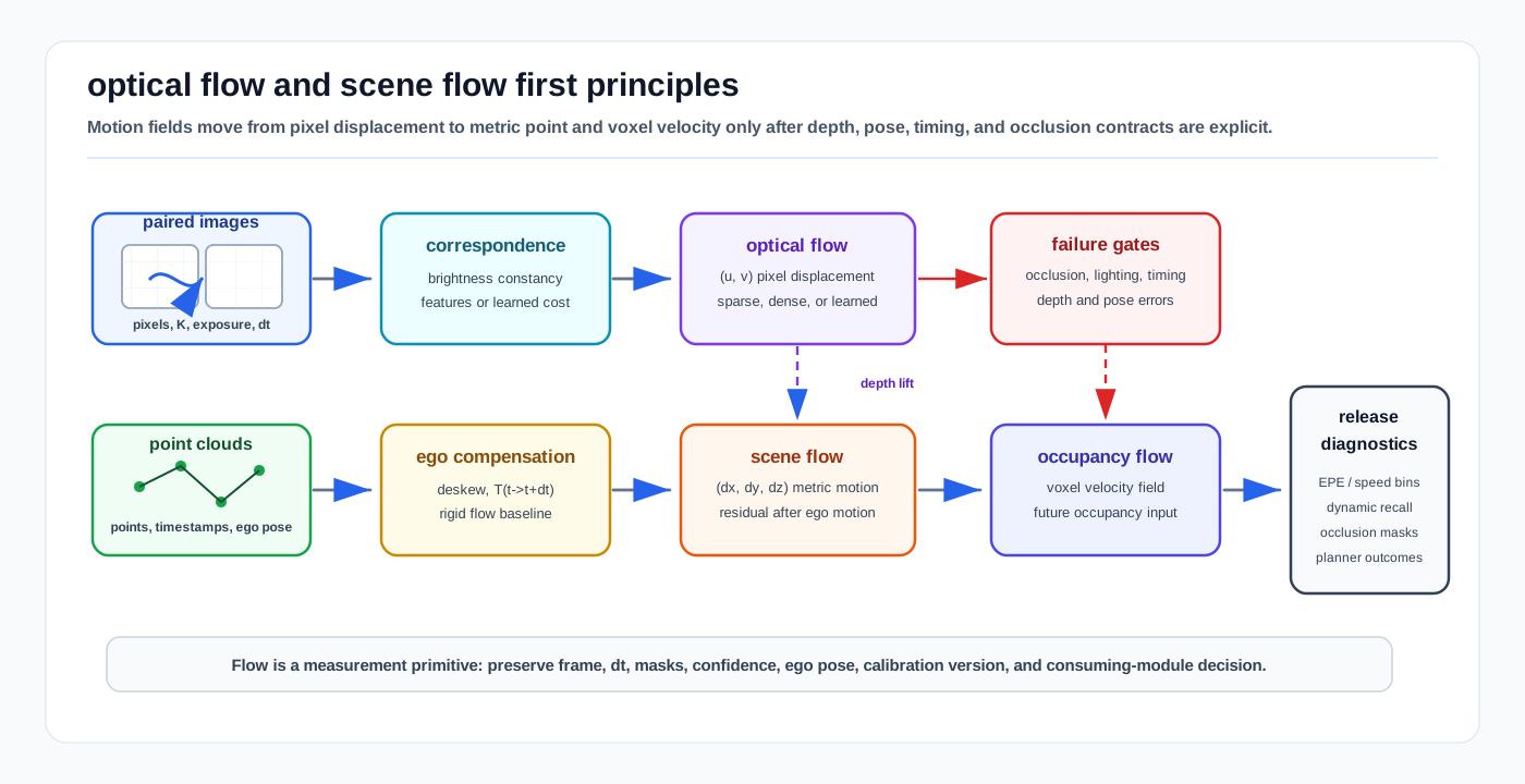
Visual: motion-field measurement chain from paired images, depth, poses, and point clouds through correspondence, ego-motion compensation, optical flow, scene flow, occupancy flow, and release diagnostics.
Optical flow and scene flow estimate motion fields before an autonomy stack has committed to tracks, object classes, or future occupancy. Optical flow is a 2D image displacement field. Scene flow lifts that idea into 3D so points, voxels, or surfaces carry metric displacement or velocity.
This page is the motion-field layer next to Epipolar Geometry, Homographies, and Two-View Verification and Camera Projective Geometry, PnP, and Triangulation. Two-view geometry asks whether image correspondences are geometrically consistent; optical and scene flow ask how pixels or points move between times, which makes them direct inputs to moving/static segmentation, occupancy flow, dynamic-map cleaning, and flow-aware planning.
1. Related Docs
- Epipolar Geometry, Homographies, and Two-View Verification
- Camera Projective Geometry, PnP, and Triangulation
- Camera Imaging, Noise, and Calibration
- Rolling Shutter, LiDAR Deskew, and Motion Distortion
- Correspondence Search and Data Structures
- Point Cloud Registration Math: ICP, NDT, and GICP
- Tracking Motion Models, Lifecycle, and Metrics
- Occupancy Flow and 4D Scene Understanding
- Scene Flow Datasets and Benchmarks
- Scene Flow for Dynamic Object Removal
- Neural Scene Flow Priors
- Cross-Domain LiDAR Scene Flow
- Self-Supervised Occupancy Flow
2. Why It Matters for AV, Perception, SLAM, and Mapping
| Workflow | Motion-field role | AV risk if wrong |
|---|---|---|
| Visual odometry and VIO | Optical flow supplies short-baseline image motion before feature tracks or bundle adjustment are accepted. | Dynamic objects, rolling shutter, or brightness changes can look like camera motion. |
| Stereo and depth completion | Optical flow plus disparity or depth change becomes image-domain scene flow. | Wrong depth lift turns a small pixel motion into a large metric velocity error. |
| LiDAR moving/static separation | Scene flow estimates residual 3D point motion after ego-motion compensation. | Timestamp, deskew, or pose errors can be misclassified as moving objects. |
| Occupancy flow and 4D world models | Per-point or per-voxel flow supervises dynamic occupancy and future-state prediction. | Flow errors propagate into conservative braking, missed crossing hazards, or map ghosting. |
| Dynamic map cleaning | Static points are retained while coherent residual flow is removed or isolated. | Over-removal can erase useful structure; under-removal fuses moving-object ghosts into maps. |
| Flow-aware planning | Velocity fields expose unknown or non-box-like motion before stable tracks exist. | Planners may treat a moving tug, pedestrian, or loose object as static occupancy. |
3. Inputs, Outputs, and Model Boundaries
3.1 Inputs
| Input | Contract |
|---|---|
| Image pair or sequence | Frames with exposure timing, camera intrinsics, distortion state, and rolling-shutter model. |
| Depth or stereo | Disparity, depth map, stereo rig baseline, monocular depth, or triangulated landmarks when lifting image flow to 3D. |
| Point clouds | Consecutive LiDAR, RGB-D, radar point, or fused point sets with timestamps and per-point sensor provenance. |
| Ego motion | T_t_to_t+dt, IMU/wheel/GNSS/SLAM pose interpolation, and scan-deskew metadata. |
| Correspondence proposal | Dense photometric matching, sparse feature tracks, nearest-neighbor point matching, learned correlation volume, or soft assignment. |
| Masks and priors | Occlusion masks, ground masks, semantic masks, static-map priors, object tracks, or valid-depth masks. |
3.2 Outputs
| Output | Meaning |
|---|---|
Optical flow (u, v) | 2D image displacement from pixel (x, y, t) to (x + u, y + v, t + dt). |
| Disparity or depth change | Change in stereo disparity or depth that lets 2D motion become 3D motion. |
Scene flow (dx, dy, dz) | 3D displacement for points or surfaces between times, usually in sensor, ego, or world frame. |
Velocity (vx, vy, vz) | Scene flow divided by dt, with frame and ego-compensation convention recorded. |
| Occupancy flow | Per-voxel motion attached to occupied grid cells or continuous occupancy fields. |
| Dynamic/static labels | Thresholded or classified residual motion after ego-motion compensation. |
| Diagnostics | Endpoint error, flow confidence, occlusion state, residual rigid-flow error, and dynamic/static precision/recall. |
3.3 Boundary With Tracking
Flow is not a track. A track has identity, lifecycle state, filtering, prediction, and association history. A flow vector only says how image evidence, points, or occupied cells moved between times. Flow can initialize or support tracks, but release evidence should not treat per-frame flow as object intent or identity.
4. Optical Flow First Principles
4.1 Brightness Constancy
For a small image displacement (u, v) over time step dt, classical optical flow starts from brightness constancy:
I(x, y, t) = I(x + u, y + v, t + dt)Linearizing for small motion gives the optical-flow constraint equation:
I_x u + I_y v + I_t = 0One equation cannot determine two unknowns. This is the aperture problem: local image evidence along an edge constrains motion normal to the edge, but not along the edge.
4.2 Lucas-Kanade Local Least Squares
Lucas-Kanade assumes flow is approximately constant in a small window W. It solves:
minimize_(u,v) sum_(p in W) (I_x(p) u + I_y(p) v + I_t(p))^2The normal equations are:
[sum Ix^2   sum IxIy] [u] = -[sum IxIt]
[sum IxIy   sum Iy^2] [v]   [sum IyIt]
The window must have enough texture in two directions. If the gradient matrix is rank-deficient, the flow estimate is unobservable or unstable.
4.3 Horn-Schunck Global Smoothness
Horn-Schunck turns optical flow into a global variational objective:
minimize_(u,v) integral (I_x u + I_y v + I_t)^2
              + alpha^2 (||grad u||^2 + ||grad v||^2) dx dy
The data term keeps flow consistent with brightness changes; the smoothness term spreads information into weak-texture regions. Smoothness is an assumption, not a guarantee. Motion boundaries, occlusions, reflections, and articulated objects violate it.
4.4 Sparse, Dense, and Learned Flow
| Family | Output | Strength | Caveat |
|---|---|---|---|
| Sparse feature flow | Motion for selected corners/features. | Efficient, good for VO/VIO and tracking. | Misses textureless, dynamic, or low-salience regions. |
| Dense variational flow | Motion for most pixels. | Useful for segmentation, depth consistency, and visualization. | Sensitive to illumination, smoothness, and occlusion assumptions. |
| Correlation-volume or transformer flow | Dense learned correspondence. | Better large-displacement and semantic matching when trained well. | Needs domain validation, confidence calibration, and geometric sanity checks. |
| Event-camera flow | Motion from asynchronous brightness-change events. | High temporal resolution and low-light fit. | Needs event-specific contrast, timestamp, and noise models. |
5. Scene Flow First Principles
5.1 Lifting 2D Flow to 3D
With depth Z_t(x, y) and camera intrinsics K, a pixel can be back-projected:
X_t = pi^-1(x, y, Z_t, K)
X_t+dt = pi^-1(x + u, y + v, Z_t+dt, K)
scene_flow = X_t+dt - T_t+dt_t * X_t
The transform term depends on convention. If the point coordinates are compared in a stable world or ego frame, ego motion must be removed. If they are compared in each camera frame, the flow mixes scene motion with observer motion.
5.2 Rigid Flow and Residual Flow
For a static 3D point, the apparent flow is caused by ego motion:
X_pred = T_t+dt_t * X_t
rigid_flow = X_pred - X_t
residual_flow = observed_flow - rigid_flow
Residual flow is the signal used by moving/static segmentation and dynamic map cleaning. It is also where many false positives enter: bad ego pose, time offset, LiDAR deskew error, or calibration drift produces residual motion even when the scene is static.
5.3 Point-Cloud Scene Flow
Point-cloud scene flow estimates a 3D vector for source points:
F: P_t -> R^3
P_t_warped = {p_i + F(p_i)}
Common objective pieces include:
| Objective piece | Role | Failure pressure |
|---|---|---|
| Chamfer or nearest-neighbor distance | Pull warped source points toward the target cloud. | Can match to the wrong repeated surface or newly visible region. |
| Cycle consistency | Require forward and backward flow to agree. | Breaks at occlusions and disocclusions unless masked. |
| Smoothness | Encourage nearby points to move similarly. | Over-smooths object boundaries, articulated equipment, and thin structures. |
| Rigid clustering | Encourage coherent object-level motion. | Fails on deformable, articulated, or partially observed objects. |
| Ego-motion compensation | Removes expected static-scene motion. | Turns localization or timing errors into false dynamics if wrong. |
5.4 Occupancy Flow
Occupancy flow maps motion to voxels or continuous occupancy fields:
O(x, y, z, t) -> P(occupied), class, flow_vectorIt is a representation choice, not a separate physical law. The flow can come from LiDAR scene flow, image-derived scene flow, object tracks, radar Doppler, or a learned world model. The release question is whether the representation preserves small, slow, thin, or partially occluded hazards enough for planning.
6. Algorithm Steps
6.1 Image Optical Flow
- Verify camera intrinsics, distortion handling, exposure timing, and resize metadata.
- Convert frames into the photometric representation expected by the method.
- Build pyramids or a coarse-to-fine schedule for large motion.
- Estimate sparse or dense flow.
- Produce confidence, residual, or forward/backward consistency masks.
- Reject or downweight regions with occlusion, glare, saturation, rolling-shutter distortion, or low texture.
- If used for geometry, cross-check with epipolar constraints and camera motion priors.
6.2 LiDAR or Point-Cloud Scene Flow
- Deskew scans and transform points into a documented source frame.
- Estimate ego motion between sweeps and remove expected static-scene motion.
- Build point correspondences, learned correlations, or an optimization objective.
- Estimate per-point flow and optional reverse flow.
- Mask occlusions, disocclusions, ground ambiguity, and low-density far range.
- Convert residual motion into dynamic/static labels only after thresholds are tied to
dt, speed, range, and pose uncertainty. - Log flow vectors, confidence, masks, ego pose, calibration version, and thresholds for replay.
6.3 Occupancy-Flow Consumption
- Voxelize or query continuous occupancy in a frame that planning consumes.
- Aggregate point or image flow into cells with uncertainty and provenance.
- Keep unknown, dynamic, static, and newly visible states distinct.
- Pass flow-aware occupancy to prediction, planning, map cleaning, or simulation with latency metadata.
- Evaluate downstream outcomes: missed dynamic hazards, false dynamic declarations, static-map ghosting, and planning interventions.
7. Assumptions and Domain Fit
| Domain | Good fit | Transfer caveats |
|---|---|---|
| Road AVs and robotaxis | Dense motion cues, object-independent dynamic detection, scene-flow benchmarks, and occupancy-flow forecasting. | Rain, glare, shadows, rolling shutter, high relative speeds, and occlusion-heavy urban scenes stress photometric and correspondence assumptions. |
| Airside autonomy | Low-speed GSE, personnel, aircraft pushback, jet-bridge motion, map cleaning, and unknown-object flow before a detector class exists. | Texture-poor apron pavement, reflective aircraft, de-icing mist, jet blast shimmer, and very slow motion require lower thresholds and sensor cross-checks. |
| Warehouses and logistics yards | Forklifts, pallets, trailer doors, dock alignment, and dynamic background removal in structured spaces. | Repeated racks and box patterns can create wrong correspondences; lighting flicker can break image flow. |
| Ports, mines, construction, agriculture | Dust-aware LiDAR flow, slow heavy equipment, terrain change, and moving/static map hygiene. | Dust, mud, vegetation motion, water spray, and deformable terrain can look like scene motion. |
| Delivery robots and campuses | Pedestrian/cyclist motion, curbside occupancy flow, and low-cost camera or RGB-D flow. | Low camera height amplifies occlusion and parallax; crowds need careful dynamic/static and identity separation. |
8. Failure Modes and Diagnostics
| Symptom | Likely cause | Diagnostic |
|---|---|---|
| Flow points in the right direction but wrong magnitude. | Depth error, stereo disparity noise, wrong dt, or unit conversion. | Plot metric velocity versus depth/range and check timestamp interval metadata. |
| Static buildings or poles appear dynamic. | Ego pose, calibration, deskew, or time synchronization error. | Recompute rigid flow from pose and inspect residual flow by range and scan ring. |
| Dynamic objects disappear into static flow. | Threshold too high, slow motion, over-smoothing, or object moving with ego direction. | Report dynamic recall by speed bucket and actor type, not only average EPE. |
| Flow bleeds across object boundaries. | Smoothness prior or voxel aggregation crosses motion boundaries. | Visualize flow discontinuities against semantic/instance masks and range images. |
| Image flow fails under lighting changes. | Brightness constancy violation from shadows, glare, HDR exposure, or thermal contrast changes. | Compare photometric residual maps to exposure, saturation, and weather metadata. |
| Newly revealed surfaces look like motion. | Disocclusion has no true correspondence in the previous frame. | Use forward/backward consistency and occlusion masks before dynamic labeling. |
| Scene flow improves EPE but hurts planning. | Benchmark metric rewards background or easy points more than rare hazards. | Add hazard-weighted, dynamic-only, small-object, and downstream planning metrics. |
| Flow confidence is high on repeated textures. | Correlation or nearest-neighbor matching found plausible but wrong surfaces. | Require geometry, temporal consistency, semantic support, or multi-sensor confirmation. |
9. Implementation Notes
- Keep the coordinate frame explicit for every flow vector. Image flow is in pixels; scene flow can be in camera, LiDAR, ego, map, or world coordinates.
- Tie thresholds to time. A 0.05 m displacement threshold over 0.1 s is a 0.5 m/s speed threshold; that can miss creeping vehicles or personnel in managed sites.
- Separate observer motion from scene motion before declaring dynamics. Rigid-flow residuals are only as good as pose, calibration, and timing.
- Preserve occlusion and disocclusion masks. Nearest-neighbor losses and forward-only flow can invent motion where no correspondence exists.
- For optical flow, document whether images were raw, rectified, undistorted, resized, or exposure-normalized. Geometry checks assume those choices are consistent.
- For point-cloud flow, log deskew settings, ego poses, point timestamps, and sensor provenance. Multi-LiDAR fusion errors often look like residual flow.
- Do not tune only on average endpoint error. Split metrics by static/dynamic, speed, range, object size, occlusion, weather, and domain.
- Treat learned flow models as measurement producers. Downstream filters and planners still need covariance, confidence, validity masks, and fail-closed behavior.
10. AV Release Evidence
Motion-field release evidence should include:
- Optical-flow evidence: photometric residuals, forward/backward consistency, texture/rank diagnostics, epipolar sanity checks, and rolling-shutter sensitivity.
- Scene-flow evidence: EPE3D or equivalent, dynamic/static precision and recall, speed-bucket splits, range splits, occlusion splits, and ego-motion sensitivity.
- Occupancy-flow evidence: future-occupancy quality, dynamic hazard recall, false dynamic declarations, planner intervention outcomes, and map-ghost reduction.
- Domain evidence: road, warehouse, yard, port, mine, farm, campus, and airside transfer splits where the same model is reused outside its source domain.
- Operational evidence: logs that preserve flow vectors, confidence, masks, ego pose, calibration version, timestamp policy, thresholds, and the consuming module decision.
11. Sources
- Berthold K. P. Horn and Brian G. Schunck, "Determining Optical Flow", Artificial Intelligence 1981 DOI record: https://doi.org/10.1016/0004-3702(81)90024-2
- Bruce D. Lucas and Takeo Kanade, "An Iterative Image Registration Technique with an Application to Stereo Vision", 1981 paper page: https://idl.uw.edu/living-papers-paper/lucas-kanade/
- OpenCV, "Optical Flow": https://docs.opencv.org/4.x/d4/dee/tutorial_optical_flow.html
- Sundar Vedula, Simon Baker, Peter Rander, Robert Collins, and Takeo Kanade, "Three-Dimensional Scene Flow", CMU Robotics Institute publication page: https://www.ri.cmu.edu/publications/three-dimensional-scene-flow-2/
- KITTI Scene Flow benchmark: https://www.cvlibs.net/datasets/kitti/eval_scene_flow.php?benchmark=scene_flow&eval_area=est&eval_gt=all
- Freiburg Scene Flow Datasets / FlyingThings3D: https://lmb.informatik.uni-freiburg.de/resources/datasets/SceneFlowDatasets/
- Argoverse 2 3D Scene Flow task: https://argoverse.github.io/user-guide/tasks/3d_scene_flow.html
- AV2 2024 Scene Flow Challenge: https://www.argoverse.org/sceneflow.html
- Waymo, "Scalable Scene Flow from Point Clouds in the Real World": https://waymo.com/research/scalable-scene-flow-from-point-clouds-in-the-real-world/
- ZeroFlow project page: https://vedder.io/zeroflow.html
- DeFlow official repository: https://github.com/KTH-RPL/DeFlow